Agentic AI for
Scientific Discovery
Reinforcement learning, model training, and research workflows.
← / → navigate · X index · N notes
Cortex: research infrastructure
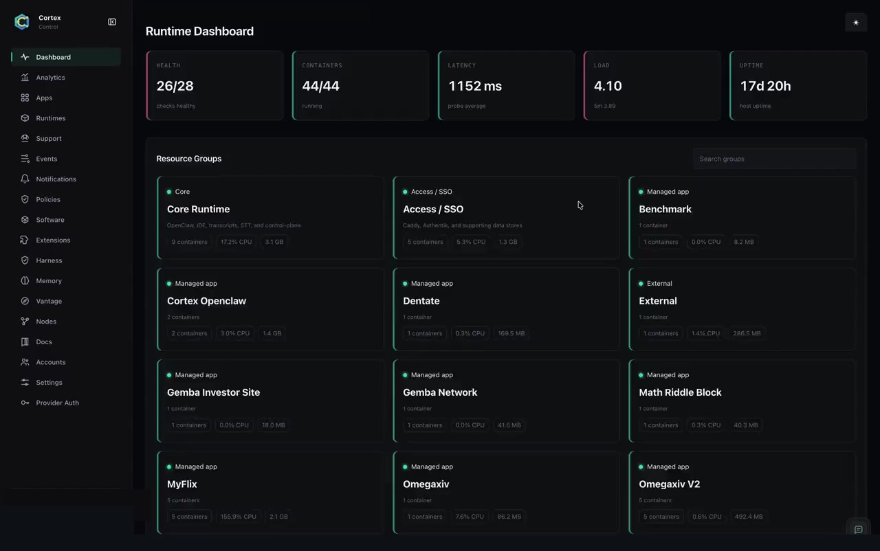

Environments, tools, access and execution records.
Public homepage · offline recording.
Control-plane excerpt at 3× speed; identifiers redacted.
Agents in scientific software
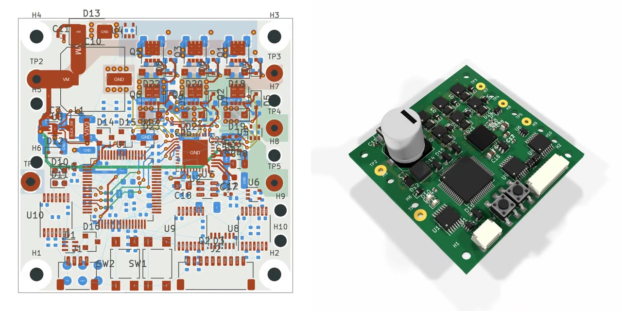
Circuit-board layout in KiCad
Component placement, routing and a 3D board view.
GPT-6 Astra, computer-use demonstration.
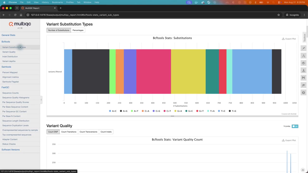
Sequencing-quality analysis
Inspection of MultiQC reports in scientific software.
GPT-6 Astra, scientific-software demonstration.
AI disproves Erdős's unit-distance conjecture
Erdős's unit-distance problem · 1946
Among $n$ points in the plane, maximize the number $u(n)$ of pairs at distance one.
Counting illustration, not the counterexample construction.
A fixed $\delta$, for infinitely many $n$.
The exact asymptotic growth remains open.
The model connected geometry to infinite towers of number fields. External mathematicians checked and simplified the proof.
Forced Navier–Stokes: claimed blow-up
$u$: velocity · $p$: pressure · $\nu>0$: viscosity · $f$: external force · divergence zero: incompressible flow

2D Taylor–Green reference flow · original animation, not the claimed 3D singularity.
Tracers follow velocity; orange/teal show opposite vorticity. Viscosity damps this flow.
Bounded total energy, unbounded peak speed. Authors claim Clay C/D; the unforced problem is not settled.
Paper + Lean formalization released. The inspected Clay page remains “Active”; formalization still needs scrutiny of the encoded statement.
Buckmaster questions use of unpublished work. OpenAI denies targeted access but cannot exclude de-identified training influence. Bubeck disputes the attribution account and apologizes for a career remark.
Automated scientific discovery
Hover to preview
Click to enlarge
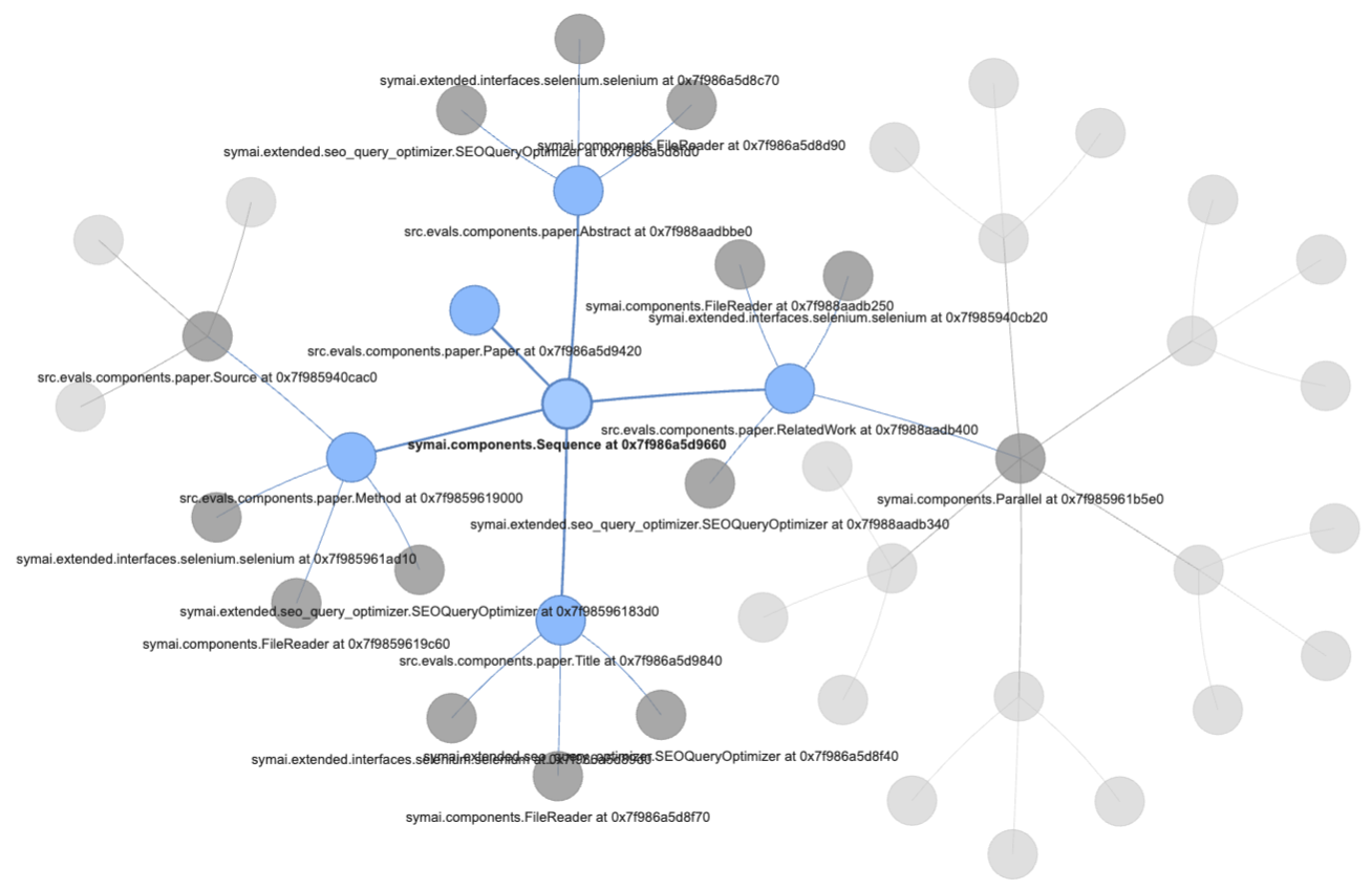
SymbolicAI
A neuro-symbolic computation graph assembles a scientific manuscript from supplied documentation and references. The benchmark evaluates intermediate and final generation outputs.
Scope. End-to-end manuscript generation—not an autonomous execution of novel research experiments.
This PhD-era work separates a complete document-generation workflow from the broader scientific process. The framework was released in January 2023; the benchmark and arXiv report followed in February 2024. Method, RelatedWork, Abstract and Title compose into Paper. A reference trajectory is an evaluation target, not evidence that the report itself was machine-written.
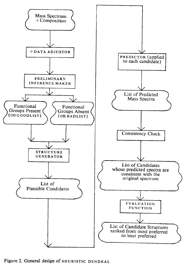
DENDRAL
Expert-guided search generates and ranks molecular structures that explain a supplied mass spectrum. The system automates a difficult step in scientific inference.
Scope. Given-data hypothesis generation—not laboratory execution or manuscript writing.
The 1969 chapter builds on Lederberg’s 1964 molecular-graph generator; a related conference report appeared in 1968. Multiple explanations could survive. The authors explicitly note that heuristic restrictions could exclude the correct structure.
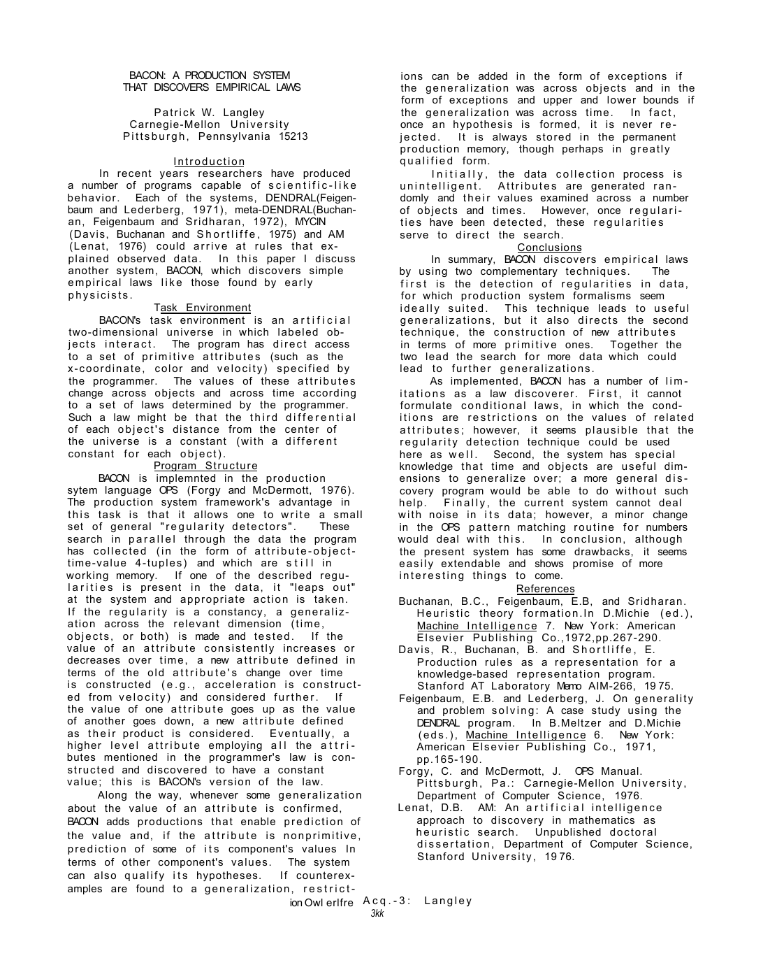
BACON
Production rules detect regularities and construct derived quantities. The original demonstration finds relationships in a programmer-defined artificial universe.
Scope. Law finding in supplied/simulated observations—not independent discovery of new physics.
Later BACON versions reconstructed familiar physical laws. Do not attribute all of those later results to this one-page 1977 report. The original implementation also assumed noise-free data.
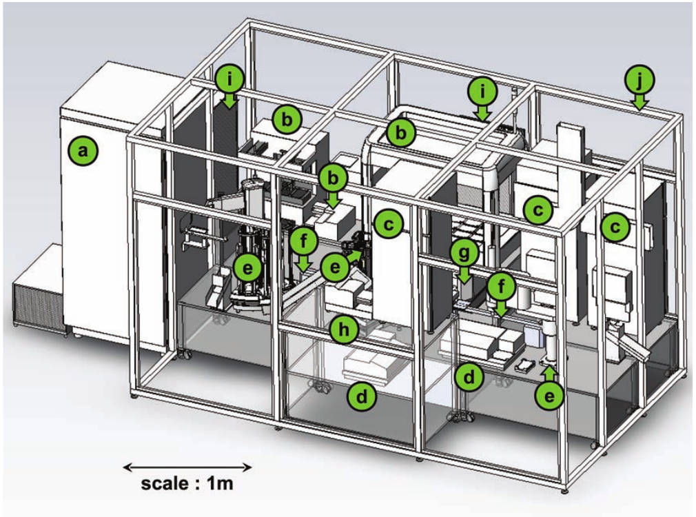
Robot Scientist
Robot Scientist and Adam connect biological hypotheses to yeast experiments, statistical evidence and machine-readable research records.
Scope. Humans supplied the study framing and infrastructure; the journal papers were human-written.
The 2004 system rediscovered known gene functions and required manual plate transfers. Adam’s 2009 study tested orphan-enzyme hypotheses and recorded a formal research argument with over 10,000 research units. Selected conclusions received independent manual checks. Physical discovery loops predate Adam, including FAHRENHEIT’s 1990 electrochemistry work.
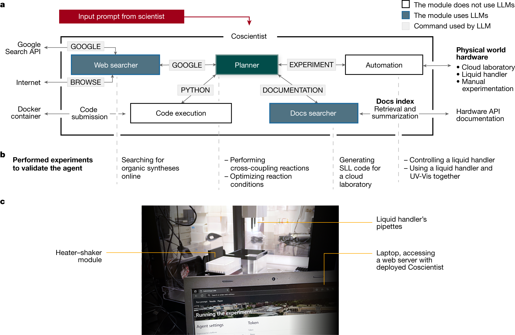
Coscientist
An LLM system uses web search, documentation, code execution and laboratory automation to plan and run bounded chemistry tasks.
Scope. Human-defined tasks and prepared lab infrastructure; some plate movement remained manual.
Demonstrations include synthesis planning, cross-coupling experiments and reaction optimization. These are experimental capabilities, not a demonstration of autonomous journal-paper generation or unrestricted scientific agency.
SymbolicAI
A neuro-symbolic computation graph assembles a scientific manuscript from supplied documentation and references. The benchmark evaluates intermediate and final generation outputs.
Scope. End-to-end manuscript generation—not an autonomous execution of novel research experiments.
This PhD-era work separates a complete document-generation workflow from the broader scientific process. The framework was released in January 2023; the benchmark and arXiv report followed in February 2024. Method, RelatedWork, Abstract and Title compose into Paper. A reference trajectory is an evaluation target, not evidence that the report itself was machine-written.
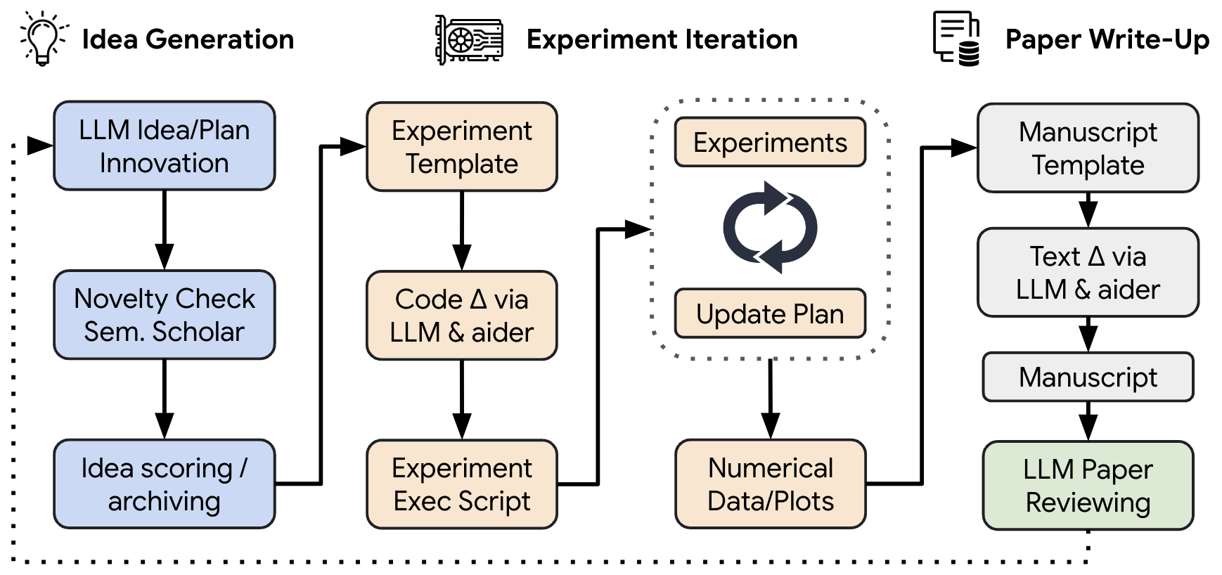
AI Scientist
A templated computational research workflow generates ideas, modifies code, runs experiments, writes papers and produces automated reviews.
Scope. Human direction and starter code constrain the domain. An automated review is not independent scientific validation.
The published demonstrations cover computational machine-learning topics such as diffusion models, language modeling and grokking. The authors report implementation errors, problematic baselines and numerical mistakes as limitations.
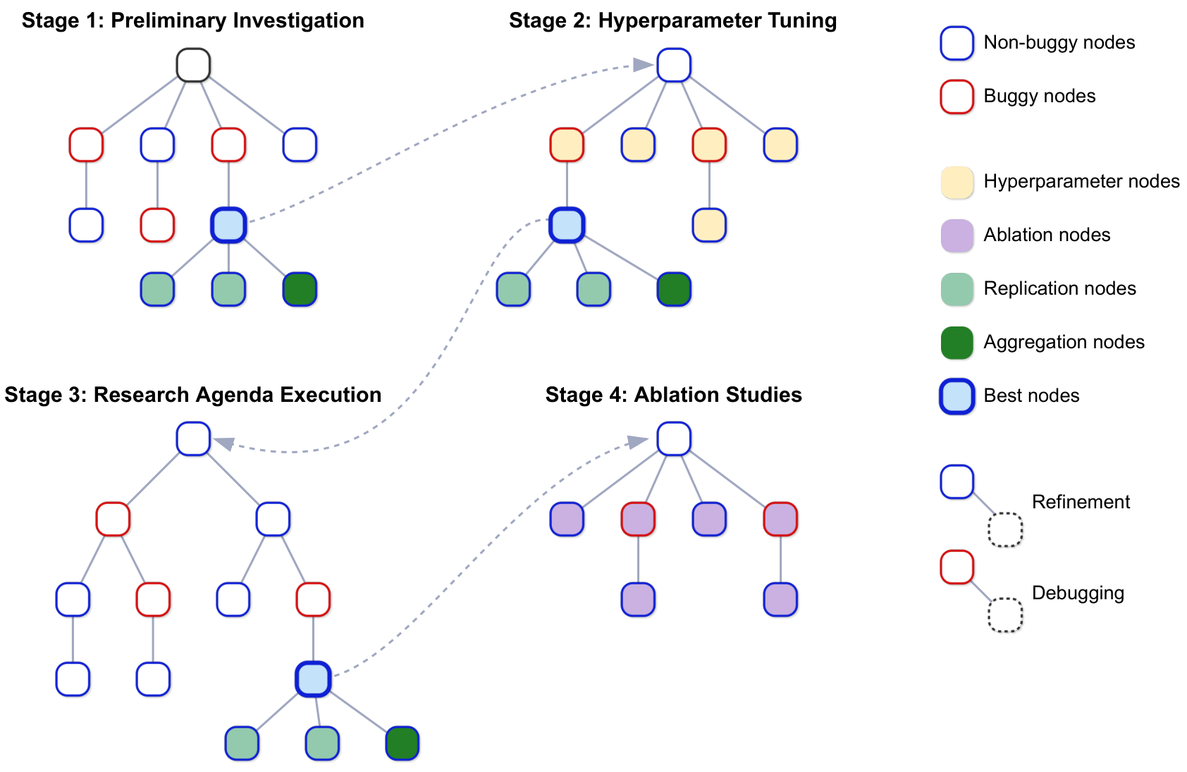
AI Scientist-v2
Experiment-tree search coordinates investigation, tuning and ablation. Selected generated papers were evaluated by external workshop reviewers.
Scope. Humans selected ideas and final runs. Workshop submissions were withdrawn before publication.
Humans selected three ideas from roughly forty candidates and chose completed runs. One of the three submissions met the workshop’s acceptance threshold, but no main-conference acceptance or publication is claimed. The paper reports no human editing of those final manuscripts, experimental code or results.
System contracts and change boundaries
"In large systems a partial understanding is the best you can do."
Sean Goedecke, July 2026
- ContractExternal behavior and invariants that must survive.
- ImpactCall paths, data dependencies and authority affected by the change.
- EvidenceTests tied to those contracts and their failure conditions.
Agent systems and
reinforcement learning
Harnesses · training objectives · controlled experiments
Agent performance: model and harness
$h_t$: observed history; $g$: goal.
$\psi$: harness configuration.
$c_t$: selected context; $\theta$: model parameters.
Context selection changes available information. Tool interfaces and permissions determine which proposals execute.
Agent harness: behavior and execution
| Harness component | Concrete mechanism | What it changes |
|---|---|---|
| Context and procedures | Markdown instructions, skills, memory selection | Information and procedural guidance supplied to the policy |
| Tool interface | MCP, tool schemas, routing and permissions | Available operations and their execution conditions |
| Persistent execution | Checkpoints, process state, budgets and stop rules | Recovery and continuation across context windows |
| Evaluation | Tests, validators and recorded environment outcomes | Which behavior is accepted and which failures remain visible |
In my setup, a Makefile assembles this configuration. Training can absorb recurring procedures; permissions and evidence checks still need external enforcement.
Durable state across context windows
| Persist | What the next work interval needs |
|---|---|
| Task state | Goal, acceptance criteria, unfinished work and explicit status. |
| Recovery state | Code / configuration versions, checkpoint and environment startup procedure. |
| Evidence and decisions | Executed checks, observed failures, rejected approaches and next action. |
Read the handoff
Restore the intended work state.
Smoke-test it
Confirm the baseline still runs.
One bounded task
Implement against its criteria.
Verify and record
Leave evidence for the next interval.
Conversation compaction is not a substitute for recoverable project state.
Repository navigation and handoffs

Path found ≠ content read ≠ scenario exercised.
“Google login works. GitHub callback is unfinished.”
Done means the user can log in and log out.
auth-v2 @ a1b2c3d
Migration 17 · npm run dev
Restore the intended state; smoke-test the running app.
“Google smoke passes. GitHub callback fails.”
Next: align the redirect URI, then rerun login/logout.
The next context reads these records.
It does not have to guess what “good progress” meant.
Artifact generation and evaluation
Save → reload → recover the same configuration.
A visible button or HTTP 200 is not this end-to-end result.
Specify the rubric before generation.
Use human-scored reference examples.
Inspect disagreements and failure traces.
Separate roles do not make their errors independent. Critique informs repair; it is not an oracle.
Planning and evidence-driven revision
Stop on acceptance or budget exhaustion.
Escalate stalled work rather than looping indefinitely.
A stronger model may need a different task size or evaluation cadence—not the same fixed ceremony.
Keep precise local acceptance criteria; avoid prescribing every future implementation step up front.
Credit assignment over tool use
$\tau$: action–observation trajectory; $p_{\theta,\psi}$: its distribution under the model and harness.
$R$: workflow reward; $\mathcal I_{\rm model}$: model-generated token positions.
$\hat A_t$: credit estimate; $\hat g$: policy-gradient estimate. On-policy samples, fixed harness and environment.
Generated tool calls and later model tokens receive credit. Tool results remain conditioning context.
Retain failures, behavior-policy scores and environment outcomes. Success-only filtering changes the learning problem.
The inference loop supplies trajectories. The training objective determines which recurring behavior they reinforce.
Workflow learning: a forecast
Elicit a procedure
Specify decomposition and response conventions in context.
Execute a procedure
Arrange tools, memory, tests and repair steps.
Learn the procedure
Optimize behavior on verified multi-step trajectories.
Task decomposition, tool selection, recovery strategies and stopping decisions.
Data access, resource authority, environment state and independent evaluation.
Current releases still co-design models and harnesses. The forecast concerns recurring heuristics, not the disappearance of execution systems.
SWE-bench scores and run costs
Verified progress · 2023–2026
Different scaffolds, budgets and sampling. The mini-SWE-agent 1.x → 2.x change is explicitly non-comparable; new vendor reports use other setups.
Run costs · latest disclosed Feb 2026
SWE-bench Pro: Opus 5 79.2 · GPT-5.6 Sol 64.6 · DeepSeek V4-Pro preview 55.4.
DeepSWE v1.1: Opus 5 68.8 · Sol 72.7 · GPT-6 Astra 74.1 · GLM-5.3 66.9 · DeepSeek V4-Pro-0813 62.7 · DeepSeek V4.1-Flash 74.2.
Provider reports; different tasks and setups, not one ranking.
METR: task-completion horizons
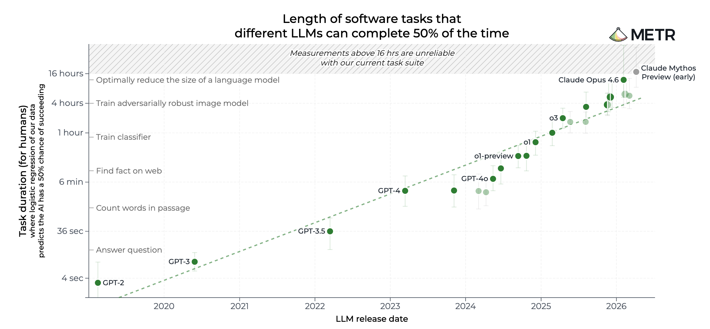
Human expert task duration, not AI runtime. Day-to-week research still needs durable state, budgets and stopping rules.
Agent training: data, rewards and updates
Fit verified successes.
22–23 · Success filtering changes the fitted distribution.
Set relative credit coefficients.
24 · RLHF reward → critic → advantage; 25–26 · Inclusive group centering.
Control the update.
27–28 · Full GRPO algorithm, advantages and KL.
Backup 46 · PPO clipping detail.
Control selection and collection.
27–29 · Grouped rollouts and estimator genealogy.
Backups 47–50 · DAPO retention and SAO collection.
Post-training objectives and supervision
Left of the dashed line an incorrect token has a defined replacement, so the objective is a cross-entropy against it. Right of it only the complete response is scored, so per-token credit must be estimated from that scalar — the subject of the remaining slides.
RLHF and RLVR: reward sources
RLHF
Reinforcement learning from human feedback
Human comparisons → fit a reward model
→ score sampled responses → update policy
Fit preferred / rejected pairs $(y_w,y_l)$; use the learned score $r_\phi$ as reward, frozen during policy updates.
Useful for taste and intent. The optimized score remains a learned proxy for human judgment.
RLVR
Reinforcement learning with verifiable rewards
Task + sampled response → execute a verifier
→ use its outcome as reward → update policy
Tests, answer checks or proof kernels supply task feedback without a learned preference model.
Binary expected reward is pass@1. Also measure pass@$k$: success within $k$ attempts can move differently.
$x$: task from a fixed distribution; $y$: response; $\pi_\theta$: policy; $r_\phi$: learned reward; $\sigma$: logistic function; $\mathcal V$: binary verifier. PPO / GRPO specify the update, not the reward source.
Success-conditioned SFT
$x$: prompt; $y$: response; $V_a$: extracted-answer verifier.
$\pi_{\rm sample}$: fixed rollout distribution; $Z_a(x)=\Pr(V_a=1\mid x)>0$.
Raw rejection samples, before deduplication or rewriting.
Each retained response supplies a teacher-forced target:
$\pi_\theta$: fitted policy; $T$: response length. Hold targets fixed.
Increase the likelihood of accepted responses.
Original STaR also uses answer-conditioned rationalizations after failed attempts. That additional proposal path is not shown here.
Success filtering favors solvable prompts
17 = 3*5 + 2
answer: 2
17 = 4*5 - 3
answer: 3
17 - 15 = 2
answer: 2
17 - 10 = 7
answer: 7
$d(x)$: proposal prompt distribution; $Z_a(x)$: answer-acceptance probability.
Equal attempts per proposed prompt; raw accepted samples pooled before deduplication.
Failed trajectories contribute no direct loss term.
Prompts with low acceptance supply few new targets, even if they matter to the final evaluation.
RLHF: rewards and advantages
At rollout time, distribute that signal over tokens:
$R_\phi$: learned response reward; $\beta$: KL weight.
$x\sim\mathcal D$ (prompts); $y\sim\pi_\theta(\cdot\mid x)$; $s_t=(x,a_{<t})$.
$T$: response length; ref: anchor; old: rollout policy.
$V_\psi$: critic; $\delta_t$: TD residual; $\gamma$: discount;
$\lambda$: GAE trace parameter; $V_\psi(s_{T+1})=0$.
If $\gamma=\lambda=1$:
$\mathbb E_{\rm old}$: rollout batch; $\epsilon$: clip width. Critic fitting is separate. Positive / negative $\hat A_t$ raises / lowers the sampled action's probability before clipping.
GRPO: inclusive group baselines
$G$: responses at one prompt $x$; $R_i$: response reward; $A_i$: mean-centered advantage.
Isolate mean subtraction before group-standard-deviation normalization.
$\hat g_{\rm seq}=G^{-1}\sum_i A_i\nabla_\theta\log\pi_\theta(y_i\mid x)$.
Iid on-policy sequences; before standardization, clipping, filtering and token normalization.
Removing the critic trades value-function learning for $G$ sampled completions per prompt.
GRPO: response-level credit
17 = 3*5 + 2
answer: 2
17 = 4*5 - 3
answer: 3
17 - 15 = 2
answer: 2
17 - 10 = 7
answer: 7
Failed responses receive negative coefficients rather than being discarded.
These coefficients encode the outcome, not the validity of each reasoning token.
Iterative GRPO: the full algorithm

$I$ outer iterations · line 3
Refresh the reference anchor; freeze it within the iteration.
$M$ batches / $\mu$ updates · lines 4–11
Collect with old; reuse fixed samples and advantages to update $\theta$.
Reward-model replay · line 12
Learned-reward iteration; not a required step for fixed RLVR verifiers.
PPO and GRPO: advantages and KL
PPO-based RLHF · learned critic
$\tilde r_t$ already includes the reference-KL cost.
The critic predicts shaped reward-to-go from each prefix; GAE supplies token-level credit.
For $\gamma=\lambda=1$: $\hat A_t^{\rm PPO}=\sum_{u=t}^{T}\tilde r_u-V_\psi(s_t)$.
Outcome GRPO · sampled group
$\mathbf R$: $G$ raw response rewards for one prompt.
One standardized coefficient per response, shared by all its tokens. No learned critic.
$(1,0,1,0)\mapsto(+1,-1,+1,-1)$ with population std.
Assume std $>0$; equal rewards give no relative signal.
$T_i$: response length; $s_{i,t}$: prompt + prefix; $a_{i,t}$: token; $\epsilon$: clip width; $\beta$: KL weight. Samples, old probabilities and $\hat A$ stay fixed.
Old sets the importance ratio; ref sets the drift penalty. KL regularization does not replace the critic's variance reduction.
Policy-gradient objective families
Dentate: experimental workbench
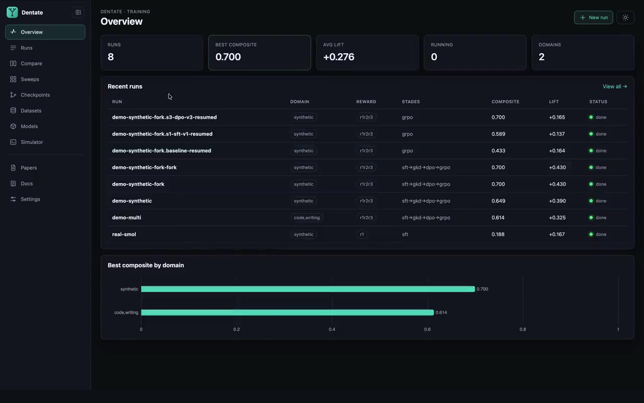
Architectures and learning experiments.
Custom models, task generators and simulation environments.
Synthetic demo data shown.
Not the Spiral measurements.
Recurrent depth and parameter sharing
$e$: encoded input; $s^{(k)}$: latent state; $R_\theta$: shared core.
$k$: iteration; $r$: number of passes; $D$: effective depth. Huginn: 3.5B unique parameters.
7M parameters, two-layer shared network.
Task-specific latent / answer refinement—not a frontier LM replacement.
TechCrunch, citing The Information, reports limited recurrent depth. OpenAI materials reviewed do not disclose an “RMM core.”
Recurrent model and training harness
$z^{(k)}$: recurrent state; $k$: iteration index.
$x$: input; $F_\theta$: shared, modulated transition.
Spiral: the recurrent model.
Dentate: the training and evaluation harness.
Historical answer-only score: 10/48 → 18/48.
Logged iterations 20–100; first point already trained.
One seed; unmatched configurations; possible earlier data overlap.
No causal attribution or current certificate-score claim.
Hosted experiment infrastructure
- Local · pip or CLI bundle
pip install "dentate[demo]", or the packaged CLI for macOS, Linux and Windows. Runs offline afterdentate demo init. - ColabOne notebook: install, run the starter experiment, then open the dashboard through the proxied port 8793. No local setup.
- VisibilityPapers, docs and results: public. Each experiment and user paper: private by default; the owner toggles it public.
Checkpoint-controlled RL comparison
pip install "dentate[demo]"
dentate demo init
dentate demo run --out my-experiment

dentate serve
# http://127.0.0.1:8793
Compare baseline and RL checkpoints on one frozen, content-disjoint task set.
SFT → support gate → GRPO from the same checkpoint → frozen evaluation. Fix decoding and loop depth. Pool construction and evaluation protocol.
my-experiment/results.json
my-experiment/metrics.json
my-experiment/provenance.json
Pre/post accuracy and the gate verdict. A failed gate is a result. Hosted alternative: /#/lab after login; private until published.
Model, data and compute controls
| Experimental factor | Actual interface | Control to record |
|---|---|---|
| Architecture | ArchSpeckey, config_factory, builder | --arch, --arch-optModel, tokenizer and checkpoint compatibility |
| Task data | ReasoningTaskid, kind, question, think, answer | --kinds modularCustom tasks through Python generators |
| Rollouts and depth | --group, --n-itersGeneration cap and decoding settings | All sampled compute Include discarded groups and skipped batches |
GRPO --steps counts attempted batches, not optimizer updates.
Changing group size changes both rollout cost and the probability of an update.
Retain run.json, metrics.jsonl and the checkpoint. Keep the acceptance evaluation outside the candidate's control.
Agentic AI for
scientific discovery
Research workflows · evidence · recursive improvement
Experience models: what to preserve
Specify the learner, the sampling law and the guarantee.
Hover or focus to inspect · click to expand
Match the conditional target mean
For a squared-loss learner with a frozen target, the expected gradient depends on its conditional mean.
$\nu$ is the common input law; $K$ is the experience kernel. Hold $Y$, target parameters and sampling laws fixed during differentiation.
Scope. Equal conditional means, under the same input law, imply equal expected gradients—not equal variance or return.
The analytic identity requires finite loss and local domination to interchange differentiation and expectation. It is a familiar conditional-expectation argument. Lean checks finite-coordinate algebra, not those analytic assumptions. If the target is differentiated, its variance can matter: for $Y=\tfrac12\theta Z$, laws $Z=0$ and $Z\in\{-1,+1\}$ with equal probabilities both have zero target mean and stopped-target update $\theta$, but full residual gradients are $\theta$ and $1.25\theta$.
Equivalence belongs to a learner
An experience model can match what a specified learner uses without reproducing the entire environment.
$\xi$ is an experience tuple; $\eta=(\theta,c)$ includes parameters and frozen context. $u$ uses the descent-sign convention.
Scope. Specify the parameter domain, sampling law and update rule. Equality of expected raw updates is not equality of training trajectories.
Context includes target networks, policies, representation, replay weights and optimizer state. A fixed replay law is not automatically the current policy’s occupancy. Equal means can coexist with different noise, and a nonlinear optimizer need not produce equal expected parameter steps. This is the study’s organizing definition, not a new general equivalence theorem.
Match the conditional target mean
For a squared-loss learner with a frozen target, the expected gradient depends on its conditional mean.
$\nu$ is the common input law; $K$ is the experience kernel. Hold $Y$, target parameters and sampling laws fixed during differentiation.
Scope. Equal conditional means, under the same input law, imply equal expected gradients—not equal variance or return.
The analytic identity requires finite loss and local domination to interchange differentiation and expectation. It is a familiar conditional-expectation argument. Lean checks finite-coordinate algebra, not those analytic assumptions. If the target is differentiated, its variance can matter: for $Y=\tfrac12\theta Z$, laws $Z=0$ and $Z\in\{-1,+1\}$ with equal probabilities both have zero target mean and stopped-target update $\theta$, but full residual gradients are $\theta$ and $1.25\theta$.
Positive alignment needs a small step
A surrogate direction decreases the reference objective only when the step respects curvature.
$g=\nabla F(\theta)$; require $\langle g,\widetilde g\rangle>0$ and $L>0$ smoothness on the entire step segment.
Scope. First-order alignment alone does not prevent overshoot. At zero gradients, cosine alignment is undefined.
The standard descent lemma bounds the change by $-\alpha\langle g,\widetilde g\rangle+\tfrac L2\alpha^2\|\widetilde g\|^2$. For $F(\theta)=\theta^2/2$, $\theta=1$ and $\widetilde g=1$, choosing $\alpha=3$ raises loss from $0.5$ to $2$ despite perfect alignment. The formal check is conditional scalar/vector algebra; it does not establish smoothness or a safe step size for neural RL.
A finite match has a finite scope
Matching a few learner states does not establish equivalence over the entire parameter domain.
For $k$ probes, $p$-dimensional updates and $N$ empirical tuples, Carathéodory gives a matching support of at most $\min(N,kp+1)$.
Scope. An existence bound—not a guarantee of optimization success, held-out fidelity, return or total-memory savings.
The convex-hull argument preserves the stacked empirical mean updates at the chosen probes. It does not prescribe a successful fitting algorithm. A uniform extension needs additional assumptions: a compact domain, an $h$-net and Lipschitz update fields. With probe error $\varepsilon$, those assumptions give a field-error bound $\varepsilon+(L_q+L_{\widetilde q})h$. Finite fitting alone does not establish them.
Lower surrogate loss can reduce return
In a terminal two-action example, biased targets reverse which action the learner prefers.
True action rewards are $(1,0)$; model training targets are $(0,1)$. Surrogate loss: $0.5\to0$. True greedy return: $1\to0$.
Scope. A constructed counterexample—not an empirical curve and not a claim that gradient matching always harms control.
The example separates descent on a model-induced objective from improvement of the actual decision problem. The same distinction motivates the next slide’s controlled measurements. Neither an optimizer trace nor a formal algebra check can substitute for a fixed, independently specified evaluation objective.
Learning outcomes and failure cases
Same law,
different learner

2.232 vs 1.712
Semi-gradient / full residual gradient.
Exact true law · 500 expected updates.
Early gain,
later deterioration

1.155 vs 0.441
Gradient matching / joint empirical.
Frozen supervised targets · test loss ↓.
CartPole:
execution evidence
Initial-check replay · 10× slow
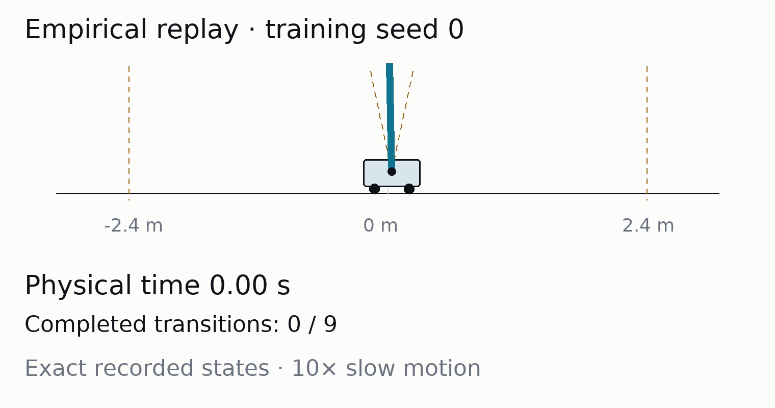
Fresh returns: 9 / 41 · two saved policies.
Not the manuscript evaluations.
49.54–86.16
Range of six method means—not an interval.
2,000 updates · 6,000 transitions/seed.
10 evaluation episodes/policy; no ranking.
From research claim to experiment

A loop-depth hypothesis
Does extra recurrence improve accuracy at fixed compute?
Require a common evaluation, versioned configurations and compute measurements.
Reject a confounded comparison. Record the revised trial before continuing.
Recorded interface, 3×. Unreviewed outputs are not results for this example.
Research artifacts and acceptance criteria
$g$: goal and constraints; $s_j$: evidence state; $a_j$: phase artifact.
$\Phi_j$: phase; $V_j$: validator returning $v_j$; $U_j$: accept, repair or escalate transition.
$E$: evidence extraction; $\mathcal A_g$: goal-dependent acceptance.
Loop-depth hypothesis → executable model/data specification → accuracy and compute measurements → accepted, rejected or revised claim.
AI-assisted model development
| Example | What the system did | What changed |
|---|---|---|
| DeepSeek-R1 Jan 2025 · Nguyen | Wrote llama.cpp WebAssembly SIMD code with human prompts and tests. | Inference software. Benchmarked on Llama; no R1 weight update. |
| PaperBench Apr 2025 · OpenAI | Claude 3.5 Sonnet: 21% average replication score across 20 papers. | Research execution. 12-hour BasicAgent; partial credit, not new findings. |
| AlphaEvolve May/Jun 2025 · DeepMind | Evolved a Gemini training-kernel heuristic: 23% faster kernel → 1% less training time. | Training infrastructure. Automatic program search; human-defined evaluation. |
| GPT-5.3-Codex Feb 2026 · OpenAI | Early versions helped debug training, analyze evaluations and manage deployment. | Its own development process. Researchers used and reviewed the assistance. |
Recursive research feedback
Nine Claude agents designed experiments and trained small Qwen students. Humans chose the problem and evaluator.
A top method's production-scale gain was within noise. Claude's own weights did not change.
Agents write code, prepare data, monitor runs and analyze results. People retain priorities and scale, pause or deploy decisions.
Internal activity and success metrics do not isolate research-productivity gains.
Autonomous recursive model improvement would require repeated successor-driven gains. These reports do not establish that full cycle or inevitable exponential growth.
Your next research question
Turn your research question
into an experiment.
Agents can help build and run it.
You decide what to ask and what counts as evidence.
Define the goal.
Define the verification.
Let the model search.
Search over architectures, training data
and experimental designs.
Choose questions, revise assumptions
and interpret the evidence.
Within two years, I expect agents to outperform much of my manual search for model and training improvements.
Questions · Open technical backup
Technical references
X: searchable slide index · B: return to the talk · N: notes
PPO: the clipped objective
$a_t$: sampled token; $s_t$: its prefix.
$\epsilon$: clip width; $\ell_t$: term to maximize.
$\hat A_t$: advantage, held fixed for the update.
The rollout policy is fixed for the batch. Several optimization passes may reuse its samples.
Both slices of the same $\min$; one bound binds per sign — $\epsilon_{\rm high}$ left, $\epsilon_{\rm low}$ right. DAPO's Clip-Higher raises $\epsilon_{\rm high}$, so it loosens the positive branch; the penalty side has no upper limit. The ratio itself is never constrained.
Reward variance and group retention
At fixed $x$, iid $R_i\sim\operatorname{Bernoulli}(p_x)$; $p_x=\Pr(R=1\mid x)$.
Binary reward; a group is retained only if its rewards are not all equal.
| At one prompt, G = 8 | Retained groups |
|---|---|
| $p_x=0.01$ | 7.7% |
| $p_x=0.10$ | 57.0% |
Half the prompts always pass.
Half always fail.
50% aggregate success.
Zero retained groups.
DAPO resamples until the batch contains enough non-uniform groups.
SAO removes the group rollout barrier
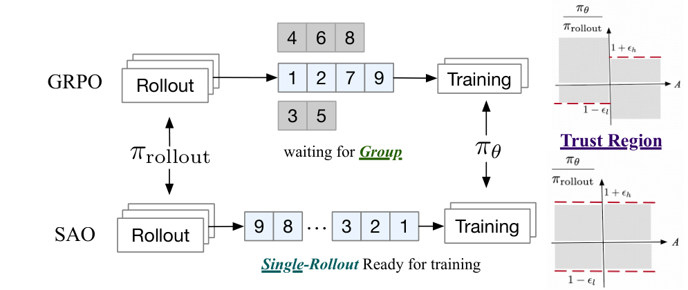
Generation order, not reward or duration.
Top: complete groups. Bottom: individual completions.
GRPO: rewards from the same prompt.
SAO: a learned token-level value function.
SAO: behavior-policy correction
$a_t$: generated token; $s_t$: its observed prefix; $\pi_\theta$: current policy.
$\ell_t^{\rm rollout}$: stored log probability at generation time.
$m_t$: policy-gradient mask; $\epsilon_\ell,\epsilon_h$: lower and upper widths.
Saturates the improving side according to the sign of the advantage.
Drops both out-of-range sides regardless of the advantage sign.
Update filtering is not a hard KL constraint. Action-boundary GAE in backup.
SAO ablations and GLM release results

DIS stabilizes the GRPO baseline.
The SAO advantage appears later in training.
Qwen3-30B-A3B; training steps, not matched wall-clock compute. Repeated evaluation is not training-seed replication.
Terminal-Bench 3.0
4.6 → 28.3
Same base model.
More environments, task diversity and post-training compute.
SAO with compaction remains in the stack. The gain does not isolate the optimizer.
Blog setup: Claude Code 2.1.207, avg@3, 400K context, 10-hour / 600-turn cap.
Answer-only versus certificate verification
Slides 23 and 26 used answer-only rewards. Now add a certificate check.
What is 17 mod 5?
Certificate: 17 = 3*5 + 1
Answer:      2
A valid certificate is 17 = 3*5 + 2, with 0 ≤ 2 < 5.
$V_a$: correct final answer.
$V_c$: valid certificate, bound to the task and answer.
Here: $V_a=1$, $V_c=0$, so $R=0$.
Answer-only: reward 1.
With the certificate check: reward 0.
Specify the accepted certificate forms; then probe rollouts against that rule.
Dense, sparse-MoE and hybrid model architectures
| Model | Execution and capacity | State / memory choice |
|---|---|---|
| Qwen3-32B 2025 · dense baseline | Dense Transformer decoder 32B parameters | Grouped-query attention KV cache grows with context |
| GLM-5.2 2026 · sparse MoE | 744B total / 40B active Sparse attention + IndexShare | One indexer per four layers Index reuse is not block recurrence |
| Nemotron 3 Ultra 2026 · hybrid MoE | 550B total / 55B active Mamba + attention + LatentMoE | Recurrent sequence state Attention layers still require KV state |
Parameter activation, context memory and repeated depth are different experimental controls.
Active weights are a compute proxy—not exact FLOPs, latency or total resident memory.
Dentate's GRPO configuration
$a_{it}$: generated token; $h_{it}$: its prefix. $\pi_{\rm ref}$: frozen starting policy.
$\mathcal M$: retained completion positions; $Z=|\mathcal M|$. Samples need not be from the current policy.
| Choice | Current local behavior |
|---|---|
| Group normalization | Mean subtraction; standard-deviation division optional. |
| Zero-variance groups | Skipped; no replacement sampling to refill the batch. |
| Token aggregation | Total retained-token mean by default (not the published fixed-length Dr. GRPO denominator); the response mean $\frac1N\sum_i\frac1{T_i}\sum_t$ is selectable, with the KL term aggregated the same way. |
| Algorithm | grpo as above, or sao: one rollout per prompt, generation-time behavior log-probabilities, value-head GAE baseline, double-sided ratio mask — a bounded single-process embodiment of SAO's components, not its asynchronous infrastructure. |
| Sampling and reuse | Temperature-adjusted sampling; raw token ratios. One inner pass by default. |
Prerequisites: package, CLI bundle, Colab or the hosted lab
Python ≥3.11 with the demo extra: PyTorch (CPU suffices), Transformers, spiral-lm and the bundled tokenizer.
Tokenizer: HuggingFaceTB/SmolLM-135M-Instruct at a pinned revision, materialized once by demo init. No download at run time afterwards.
pip install "dentate[demo]"
dentate demo init     # tokenizer + starter project
dentate demo doctor   # torch / spiral / tokenizer
dentate demo run --out my-experiment
dentate serve         # http://127.0.0.1:8793
No Python: the CLI bundle for macOS arm64, Linux x64 and Windows x64 runs the same commands. Colab proxies port 8793.
my-experiment/results.json     # pre/post accuracy, gate
my-experiment/metrics.json     # curves
my-experiment/provenance.json  # configuration lineage
my-experiment/result.dentate   # importable package
Re-evaluate the RL checkpoint with the same task set and decoding settings as the baseline.
The generic dentate run development example is fake-backed. It is not the real Spiral training exercise.
Hosted: /#/lab after Authentik login; experiments queue on CPU worker containers and stay private until published.
Public, no account: documentation · Spiral technical report · published results
Scientific workflow: artifacts, validation and acceptance
$g$: goal and constraints. $s_j$: evidence / artifact state entering phase $j$.
$\Phi_j$: proposing phase. $a_j$: its output artifact. $V_j$: validator; $v_j$: verdict.
$U_j$: state transition, including bounded repair or escalation.
$E$: collect results and provenance. $e_t$: evidence from trial $t$.
$\mathcal A_g$: predeclared acceptance rule for goal $g$, not a guarantee of truth.
RL additionally updates a policy from a reward signal.
Content-disjoint evaluation for the modular task
from dentate.pretrain.reason_run import (
    sample_mixed, sample_heldout,
)
key = lambda t: (t.kind, t.question, t.answer)
sft = sample_mixed(2048, seed=0, kinds=["modular"])
rl = sample_mixed(512, seed=0, kinds=["modular"])
excluded = {key(t) for t in sft + rl}
heldout, missing = sample_heldout(
    48, seed=200000, kinds=["modular"],
    exclude=excluded,
)
assert heldout
assert not ({key(t) for t in heldout} & excluded)
print("Evaluation denominator:", len(heldout))
Freeze these tasks before inspecting either model's score.
Use the same ReasonTrainer.evaluate call for each checkpoint: same tasks, tokenizer, system prompt, loop depth and 48-token budget.
Only 760 possible modular questions in this generator. The remaining set may be small. Report it.
Support, answer accuracy and valid trace format are separate measurements.
Myflix: a personal media service

A streaming service I control.
Library, playback, deployment
and Android TV.
Edited navigation recording.
Recoverable experimental state
Day-to-week
research tasks.
Search loop depth and data under a fixed budget. Reproduce the strongest candidate across seeds on untouched tasks.
Recover code, configuration, checkpoints and rejected hypotheses across context windows.
| Failure mode | Required control |
|---|---|
| Context exhaustion | Durable artifact and decision state |
| Interrupted tools | Actual process state and safe resumption |
| Delayed outcomes | Intermediate checks tied to the final objective |
| Human redirection | Versioned goals, budgets and acceptance criteria |
Stop on acceptance, budget exhaustion or a recovery decision that needs human input.
Supervised initialization and rollout evaluation
$y^*$: supplied target; $\mathcal M$: its supervised output-token positions.
Training uses target prefixes. Rollout uses sampled prefixes.
SFT is one route to reward-bearing rollouts, not a universal prerequisite for RL.
Probe the rule chosen on backup 51; report answer-only success separately.
Token-level and response-level loss weighting
$\rho_{it}$: current / rollout-policy probability ratio; $A_i$: response advantage.
$N$: retained responses; $T_i$: generated-token count. Prompt / environment tokens excluded.
Longer responses carry more aggregate token weight.
Each response average has the same coefficient.
Filtering changes the retained population. Specify it together with the denominator. The Dentate demo exposes both aggregations (loss_aggregation), the advantage normalization, the clip band and a bounded single-process SAO (algorithm); its weighting.json records the per-response terms so both means can be recomputed by hand.
Controlled RL comparisons
$A$, $B$: baseline and treatment; $x_j$: shared held-out task.
$V$: fixed acceptance rule; $y_j^A,y_j^B$: outputs under a matched decoding protocol.
| Control | What must be comparable |
|---|---|
| Initialization and data | Same starting checkpoint and training task distribution. Audit test overlap across every training stage. |
| Evaluation | Frozen tasks, verifier, decoding and token caps. Select checkpoints on development data, not the final test set. |
| Compute and uncertainty | Matched budget, including discarded samples. Repeat training seeds; report paired task effects and seed variation. |
Task distributions and verifiers
| Task and artifact | Automated feedback | Unresolved validity |
|---|---|---|
| Code change Patch and execution trace | Behavior, regressions, permission boundaries | Untested cases and system-level effects |
| Video edit Timeline and rendered output | Synchronization, required assets, render constraints | Meaning, pacing and narrative intent |
| Simulation Model and trial specification | Numerical consistency, constraints, repeatability | Modeling assumptions and real-world fidelity |
Task generator + admissible artifacts + verifier + evaluation protocol
form a reusable environment for domain-specific model improvement.
SAO advantage estimation across tool observations
Final generated token
$a_{i,N}$
Conditioning context
No intermediate GAE steps.
First generated token
$a_{i+1,0}$
$a_{i,N}$: final token of action $i$; $a_{i+1,0}$: first token of the next action.
$V$: critic at the indicated token's prefix; $r$: reward; $\gamma$: discount; $\lambda$: GAE decay.
$\delta$: temporal-difference residual; $\hat A$: advantage estimate.
Observation tokens remain in context, but not in the generated-action recursion.
The action boundary uses one discount step. Terminal bootstrap and continuation are zero.
Long-horizon training infrastructure
| Component | What changes | Evidence boundary |
|---|---|---|
| SAO | Single rollouts, DIS, critic training and observation-skipping GAE | Qwen3-30B-A3B study; not a GLM optimizer ablation |
| slime | Megatron training, SGLang rollouts, buffer and environment interfaces | Training infrastructure; not an advantage estimator |
| Compaction | Variable-count, variable-length sub-trajectories in long tasks | GLM release training design; not isolated by the paper's tables |
| IndexShare | Reuse sparse-attention indices across four layers | Architecture / inference efficiency; not recurrent-depth weight sharing |
SAO paper: 128k budget; math ≤50 turns, coding ≤300 OpenHands turns.
Math evaluation repeats: 16 for AIME / HMMT / IMOAnswerBench, 4 for BeyondAIME.
Reward sources and costs in LLM post-training
An agent is a policy whose actions change the state it will next observe.
Not a slogan — a checklist. Four properties are needed before the word carries information, and the missing property tells you which failure mode a system has.
A system is agentic to the extent that it is a policy $\pi$ acting in an environment: it emits actions $a_t$ with external effects, receives observations $o_{t+1}$ that depend on those actions, carries state across steps, and terminates against a goal. Formally, a POMDP $(\S,\A,\mathcal{O},P,r,\gamma)$ — the object from Day 1, with $\S$ hidden.
Each property is an experiment you can run: perturb the environment, check whether behaviour changes. Systems that fail the test do not need RL, and RL cannot help them.
Policy gradients for the token-level MDP
- +Deterministic dynamics → no environment model
- +Known likelihood → importance ratios for free
- −One scalar after $10^3$–$10^5$ decisions → credit assignment breaks
Verification cost in the reward objective
Published objectives set $c\equiv0$. Fine where the checker is free — math, code. Not fine where an instrument is involved.
Sequence-level bandits and token-level MDPs
Sequence = one arm (bandit)
The reward is a single terminal scalar, so treat the whole response as one action. No per-token value function, no per-token ratio; the baseline is the mean reward of other samples for the same prompt.
- +Matches the unit of the reward; importance weight is a single, well-defined ratio
- +No critic to train, no critic to be wrong
- −No mechanism to distinguish a decisive token from a filler token
RLOO · GSPO · REINFORCE-style group methods
Sequence = $T$ actions (token MDP)
Keep the full MDP: per-token advantages, a value function over prefixes, and credit assignment inside the response. DPO admits a token-level reading as inverse $Q$-learning satisfying a Bellman equation.
- +Credit assignment inside a chain of thought becomes expressible
- +Search over prefixes (MCTS-style) becomes well-defined
- −Per-token ratios are single-sample estimates: variance accumulates over $T$ and clipping amplifies it
PPO-RLHF · token-level DPO · process-reward methods
The token-level objective is a first-order approximation of the sequence-level objective, exact iff $\pit=\piold$. Every deviation from strict on-policy sampling — mini-batching, asynchronous rollouts, an inference engine with different kernels — makes the approximation worse. Part III is largely a catalogue of that fact.
Reward maximization with a reference-policy KL penalty
- 1Sample it — PPO, GRPO: Part III
- 2Cancel it — DPO (backup)
- 3Approximate it — best-of-$n$, mirror descent
Control: a trust region around where $r$ was fitted. Inference: posterior sampling, not utility maximization.
Sampled KL estimators: bias, variance and sign
With $\rho=\piref(y_t\mid\cdot)/\pit(y_t\mid\cdot)$ evaluated on samples from $\pit$, three estimators of $\KL[\pit\|\piref]$ are in circulation. They differ in variance and in whether a single sample can come out negative.
Unbiased. High variance, and negative for roughly half of samples — an estimate of a non-negative quantity that is negative half the time is a poor training signal.
Always non-negative, low variance, biased. Bias vanishes as the policies converge; in practice the bias is small compared to k1's variance.
Unbiased and non-negative for every sample, since $\rho-\log\rho-1\ge0$ with equality at $\rho=1$. This is the estimator written into the GRPO objective, and what most frameworks ship.
Near the reference ($\rho\approx1$) every estimator is a difference of nearly equal numbers, and the sign-indefinite k1 injects its noise straight into the gradient. Scaling by $\beta$ scales that noise with it — a larger $\beta$ makes the KL term matter more, not the estimator matter less. k3 is bounded below by zero, which is why it survived.
Whether to keep a KL term at all in verifiable-reward RL is contested: several 2025 recipes (DAPO among them) remove it, arguing the policy is meant to move far from the reference during long-horizon reasoning training. Removing it also removes the only thing bounding the drift.
Credit assignment over $10^3$–$10^5$ decisions
- 01Critics degrade — a policy-sized value head, trained on a reward that exists only at $t=T$
- 02Broadcasting wastes gradient — the decisive step and the whitespace after it get the same credit
- 03An oracle critic can hurt — it penalizes the wrong branch that error-then-recovery needs (Kimi)
Reward redistribution (RUDDER): a dense reward with the same optimal policies, credit given to the steps that shifted the expected return. Largely unexploited in LLM post-training.

Chain of thought = demonstration trajectory. Verifier score = delayed return.
In the published 2025–26 pipelines, reinforcement learning appears in three of the five post-training stages.
Next-token prediction on $10^{13}$ tokens. Defines the support of everything downstream.
no rewardFormat, instruction following, long-context and tool syntax; distillation from a stronger teacher.
imitationHuman or AI preferences via a reward model, or offline via DPO-family losses. Style, safety, refusals.
learned rewardMath, code, formal proof: reward is a checker, not a model. The stage that produced "reasoning models".
programmatic rewardMulti-turn tool use in real environments: browsers, shells, repositories, simulators. Reward at task completion.
environment reward2022: one RLHF pass, tiny compute, style objective. 2026: multiple RL stages, a substantial fraction of post-training compute, and objectives that are checkable rather than preferred.
The estimator. It is still a score-function gradient with a baseline and a trust region. The innovation is on the reward and infrastructure sides.
Each stage narrows the distribution the next one explores. RL cannot recover a capability that pre-training never put in the support — which is precisely the Part IV controversy.
SFT maximizes the likelihood of a fixed target; RL reweights the model's own samples by a score.
- →Weaker supervision suffices. A verifier that says yes/no is far cheaper than a demonstration, and exists for whole domains where demonstrations do not.
- →Distribution match. RL optimizes the object you deploy: samples from $\pit$, under the decoding policy you will actually use.
Generalization: in matched comparisons on rule-based and visual out-of-distribution variants, RL post-training transferred while SFT largely memorized the training format — with the important qualifier that SFT was still needed first to make outputs parseable enough for RL to start.
Forgetting: on-policy RL fine-tuning was found to reach comparable task performance while incurring a smaller KL shift from the base policy than supervised fine-tuning, and correspondingly less degradation on held-out abilities.
Most such comparisons are (i) on a small number of model families, (ii) at a fixed compute budget that favours one method, and (iii) evaluated with pass@1, which is exactly the metric Part IV shows can move without capability moving. Treat "RL generalizes, SFT memorizes" as a well-supported tendency, not a theorem.
Comparing trajectory, reward and infrastructure choices
The 2024–26 methods are easier to compare along three axes than chronologically. Most published variants move one axis and inherit the rest; naming the axis indicates what the method can and cannot fix.
How do samples enter the update?
Group size $G$, dynamic sampling and difficulty filtering, ratio granularity (token / sequence), clipping asymmetry, loss aggregation over tokens or sequences, staleness tolerance.
GRPO · RLOO · DAPO · GSPO · CISPO
What weights the update?
Learned reward model, rule verifier, execution, process reward, rubric or judge; the baseline (critic, group mean, leave-one-out); normalization choices and the biases they inject.
RLHF · RLVR · PRMs · rubric rewards
Which policy actually produced the data?
The rollout engine and the training engine disagree numerically; rollouts are asynchronous and stale; the "on-policy" objective is silently off-policy. Staleness was known in classical distributed RL (IMPALA's V-trace); the engine mismatch is new.
truncated IS · async RL · partial rollouts
Reward sources, evaluation costs and failure modes
The latent scalar-utility assumption in RLHF
Actor $\pit$ (updated), critic $V_\psi$ (updated), reward model $r_\phi$ (frozen), reference $\piref$ (frozen). The critic scores partial generations, the reward model scores complete ones — they are different objects and are routinely conflated.
Reward models are trained on comparisons drawn from a narrow policy. Once RL moves the policy, the model is evaluated off its training distribution — and its accuracy there is not measured by the validation loss that was used to select it. Ranking accuracy of most preference-tuned models is below 60 %, and correlates with win rate only near $\piref$.
Fitted overoptimization laws for best-of-$n$ and RL
- →Best-of-$n$ is KL-cheap: $\KL_{\text{bo}n}=\log n-\tfrac{n-1}{n}$
- →RL is not: KL grows ~quadratically in steps — a poor common currency
- →The KL penalty is early stopping: it does not move the KL–gold frontier
Overoptimization is a budget: from the proxy-RM size, predict the distance where gold peaks — and stop there.
Each reward source in this table has at least one documented exploit.
A learned reward inside an RL loop is an attack surface; a programmatic reward moves the attack to the specification. Neither removes the problem — they relocate it to where you can or cannot audit it.
DPO: closed-form preference objective
With implicit reward $\hat r_\theta(x,y)=\beta\log\frac{\pit(y\mid x)}{\piref(y\mid x)}$, the DPO loss is the reward-model loss — fitted in a family whose optimal policy is the model itself. Theorem 1 of the paper shows the parameterization is lossless: it fixes the gauge freedom $r\mapsto r+f(x)$ by selecting the normalized representative.
A contrastive update with an adaptive weight that vanishes once the pair is confidently ranked — which is also why DPO struggles to flip pairs the reference already ranks wrongly.
Direct-alignment objectives and inherited limitations
Offline and on-policy preference optimization
$\Pi_{\text{PPO}}\subsetneq\Pi_{\text{DPO}}$: every solution of the KL-regularized RL problem is a DPO solution, but not conversely. DPO can assign probability mass to responses never observed in the preference data, because nothing in the loss constrains behaviour off the annotated pairs.
On competitive programming (CodeContest), a verifiable domain with no judge in the loop, the PPO-trained policy reaches 22.4 % 10@1k against the previous state of the art (AlphaCode-41B with clustering, 16.4 %) — while in the same study the DPO family collapses to 0.0 % (DPO) and 3.2 % (iterative DPO).
On-policy sampling makes the model's own current errors the training signal. Offline data makes someone else's errors the training signal — and those become less relevant with every gradient step.
Reverse-KL-regularized on-policy training is mode-seeking: it concentrates on a subset of good behaviours. Maximum-likelihood-style offline objectives are mode-covering: they spread mass, including onto low-quality modes present in the data.
PPO-versus-DPO results are extremely protocol-sensitive: reference model, data source, epoch count, and whether the preference data was generated by the same policy being trained. A study that reuses public offline pairs is testing a different question from one that regenerates pairs on-policy.
RLVR: programmatic rewards
Accuracy — rule-based check of the final answer. Format — the reasoning inside the required tags. No reward model, no PRM, no MCTS.
"Once a model-based PRM is introduced, it inevitably leads to reward hacking."
A sudden rise in the frequency of the token "wait" — and response length growing without being rewarded.
Nature version: 77.9 %. Preprint: 71.0 %, same curve.
Verifier coverage, cost and claim strength
Process supervision in reranking and RL
Step-level supervision beats outcome supervision for selecting among candidate solutions: 78.2 % versus 72.4 % of MATH test problems solved when reranking with a process- versus outcome-supervised reward model. The PRM800K dataset — 800k step-level human labels — is the reference artefact.
Math-Shepherd replaces human annotation with Monte-Carlo rollout estimates of step correctness, making PRMs cheap. The lesson from later analyses: those labels measure completability, not correctness, and the two come apart precisely on the steps that matter.
DeepSeek-R1 lists PRMs under unsuccessful attempts: step definition is unclear, labels do not scale, and "once a model-based PRM is introduced, it inevitably leads to reward hacking". Math-Shepherd itself reports step-level PPO gains — the claim is about frontier-scale RL, not about PRMs as such.
A benchmark that looks discriminative (BoN, 61.6–69.3 across all models) hides a spread from 9.7% to 58.1% — a 6× range — in the ability these models were built for; choosing a PRM by BoN score selects almost at random. Today PRMs survive as inference-time rerankers and step-level error localizers, not as RL reward functions.
Rubric rewards, generative reward models and reward hacking
Write explicit, weighted criteria; have a model grade against them; use the aggregate as the scalar. Reported: rubric rewards extend RLVR-style training into medicine and science and improve alignment with human preferences across scales, with expert-written guidance crucial for synthetic rubric quality.
Rubicon: with only ~5k training samples, +5.2 points absolute on open-ended benchmarks for a 30B MoE, and +2.4 points over a 671B reference model on those benchmarks — self-reported.
Let the reward model reason before scoring, and scale it at inference: principle generation plus critique, with voting over samples. DeepSeek-GRM reports 69.9 greedy → 71.0 at voting@32 → 72.8 with a meta-reward model — inference-time scaling applied to the reward, not the policy.
Seesaw effect: jointly training strict constraint-following and open-ended creativity reduces overall performance — conflicting objectives, mitigated only by stage-wise training.
Rapid hacking: reward hacking emerged early enough to require an offline analysis of anomalously high-reward rollouts, distillation of the recurring patterns into a dedicated reward-hacking-defence rubric, and its insertion as a veto constraint in all later stages.
A veto constraint is a confession: linear scalarization of criteria is hackable, so the fix is a hard filter rather than a better weight. Expect the same pattern anywhere a learned judge sits inside the loop.
Choosing rewards by checkability, horizon and error cost
What does a wrong reward cost? If the answer is a poor chat response, train and iterate. If it is a retracted paper, damaged beam time, or a synthesized compound, the verifier should be validated before it is optimized — and that validation is itself a research task.
All of Part II fixed what weights the update. Part III is about how the samples enter — where the last three years of algorithmic work actually happened.
PPO clipping and trust regions
No monotonicity guarantee; behaviour depends on $\varepsilon$, on how many inner epochs are run per rollout ($\mu$), and on whether the sampler matches the trainer. All three are engineering choices that the theory does not cover.
It must match the actor in capacity, is trained from a reward that exists only at $t=T$, and is hard to make accurate per token when only the last token carries a reward. That is DeepSeekMath’s stated reason for removing it — not memory alone.
GRPO: critic-free, group-relative policy updates
- =REINFORCE with a group-mean baseline — RLOO up to $G/(G-1)$
- KLk3 estimator in the loss, not in the reward — the advantage stays clean
- !The two normalizers change the objective — length and std biases (backup)
$G=64$, one update per rollout ($\mu=1$). GSM8K 82.9→88.2, MATH 46.8→51.7, DeepSeekMath 7B.
How reward and length normalization change loss weighting
With $\adv>0$ (correct), dividing by $|o_i|$ gives larger updates to shorter responses. With $\adv<0$ (incorrect), longer responses are penalized less. Net effect: correct answers get shorter, wrong answers get longer.
This is the mechanism behind "GRPO grows response length": at least partly an optimization artefact, not emergent deliberation.
Dividing by $\operatorname{std}(\mathbf r)$ per question up-weights questions whose rewards are nearly all 0 or nearly all 1 — exactly the uninformative ones. Batch-level normalization would not do this; question-level normalization does.
def masked_mean(tensor, mask, dim):
-   return (tensor * mask).sum(dim) / mask.sum(dim)
+   return (tensor * mask).sum(-1) / MAX_TOKENS
Template, not RL. Qwen2.5-Math-7B average: R1 template 0.0, Qwen template 26.5, no template 38.2. A prompt-format choice moves the score more than most RL ablations.
"Aha" is not emergent. Self-reflection keywords are present in base models, including DeepSeek-V3-Base, before any RL — measured over 40,000 responses; nearly half the self-reflecting responses are no more accurate than the rest.
Removing $\operatorname{std}$ trades bias for variance; on Qwen3 base models at small reward scale, group-level normalization is reported to be the most stable choice. Method choices here are not universal.
Naive GRPO scored 30 on AIME. The same estimator with four fixes scored 50.
- 1Clip-higher ($\varepsilon_{\text{low}}{=}0.2$, $\varepsilon_{\text{high}}{=}0.28$): symmetric clipping caps low-probability exploration tokens far more tightly than high-probability exploitation tokens.
- 2Dynamic sampling: drop all-correct and all-wrong groups — their advantage is identically zero, so they contribute noise and no gradient.
- 3Token-level loss: normalize by total tokens in the batch, not per response — long low-quality samples can then be penalized properly.
- 4Soft overlong punishment: a graded length penalty in a cache band instead of a hard truncation, so a sound-but-long proof is not scored as wrong.
"The final reward on the training set often exhibits little correlation with the accuracy on the validation set" — i.e. overfitting to the training set is visible in their own runs.
Techniques do not compose additively: in one study a two-technique recipe outperformed a six-technique one.
Exactly two modifications to the critic-free PPO loss: (i) advantage normalization with a group-level mean and a batch-level standard deviation; (ii) token-level loss aggregation. Reported to outperform the six-technique DAPO recipe and GRPO on their models.
- →Clip-higher helps aligned models and can damage base models. Base models operate at a policy clipping rate around 0.003 — there is almost nothing to unclip.
- →Which tokens get clipped is linguistic: at $\varepsilon_{\text{high}}=0.2$ clipping concentrates on connectives — "therefore", "if", "but"; raising it to 0.28 shifts clipping toward high-frequency function words.
- →Std-normalization hurts on easy data: a small denominator amplifies gradients on extreme-difficulty items and can trigger gradient explosions.
Model family, alignment state, reward scale, response-length cap and data difficulty all flip the sign of individual tricks. The DAPO ladder is a Qwen2.5-32B-base result; the Lite PPO result is Qwen3-4B/8B. Neither generalizes by default.
The Lite PPO paper reports training curves, not tables: there is no numeric results table to quote. Any bar chart of its results would be fabricated — which is why this slide has none.
GSPO sequence-level importance sampling
$s_i=\exp(\overline{\log w})$ is a geometric mean of per-token ratios, not the sequence importance weight $\prod_t w_t$. GSPO is a deliberately biased surrogate chosen for bounded variance — the paper argues from variance, not from unbiasedness.
GRPO's per-token ratio is computed from a single sample of each next-token distribution. With $N=1$ it cannot perform distribution correction; it injects high-variance noise that accumulates over sequence length and is amplified by clipping.
In a sparse mixture-of-experts model, a small parameter update can change which experts are routed, so per-token likelihood ratios move discontinuously between rollout and update. Sequence-level ratios average that away; the alternative was Routing Replay, i.e. pinning the routing.
A variant that restores per-token advantages while remaining numerically identical to GSPO when all tokens in a response share one advantage — the hook for multi-turn and tool-use settings in Part V.
Clipping removes the gradient from rare tokens — reported to be the reflection markers in long reasoning traces.
Tokens with large importance ratios are the ones that were rare under the old policy: reflection markers such as "However", "Recheck", "Wait", "Aha". PPO-style clipping zeroes their gradient contribution — the update systematically discards the tokens that change the trajectory of a proof.
where $\sg[\cdot]$ blocks gradient flow through the weight, $\rho_{i,t}$ is the usual token ratio and $\adv_i$ the group-relative advantage.
In the MiniMax-M1 report, CISPO reaches the same performance as a DAPO-style baseline in roughly half the training steps in their matched setting, with the full RL run disclosed at $534,700 — an unusually concrete cost disclosure. self-reported
DAPO widens the clip window; CISPO replaces clipping with weight truncation. Both concede that the vanilla PPO clip is mis-specified for long reasoning traces, and both are bias-for-stability trades.
MiniMax reports clip-higher was less effective in their setup — 16 off-policy update rounds per generation batch. The number of inner epochs $\mu$ silently changes which trick works.
Mirror-descent targets for policy regression
The optimizer is reset at each outer iteration, because the reference — and therefore the optimization problem — changes. Length is controlled by an explicit reward term rather than by loss aggregation.
Long-CoT model: MATH-500 96.2, AIME 2024 pass@1 77.5, LiveCodeBench 62.5, Codeforces percentile 94. RL context window scaled to 128k. self-reported
No ablation isolates the $\ell_2$ proximal term against clipping. The claim "mirror descent beats PPO-clip" is not established by this paper — it is an alternative with a clean derivation.
Inclusive and leave-one-out group baselines
Policy lag and numerical mismatch in rollout training
A rollout batch is split into minibatches: $\mu=B_{\text{train}}/B_{\text{mini}}$ gradient steps are taken against samples from a policy that no longer exists after the first one. DAPO runs $\mu=16$; DeepSeekMath ran $\mu=1$. The same objective at $\mu=1$ and $\mu=16$ is a different algorithm.
The rollout engine (vLLM/SGLang, fused kernels, different batching) and the training engine (FSDP/Megatron) assign different probabilities to the same token under the same weights. The policy that generated the data is literally not the policy being updated, even at $\mu=1$.
The sequence weight is a product of $T$ token ratios. If each token contributes a small $\chi^2$ divergence, the variance of the product grows like $(1+\chi^2)^T-1$: exponential in length. Clipping each factor bounds the factors, not the product.
Two labs running "the same" GRPO can differ by more than any published algorithmic delta, purely through $\mu$, engine pairing, and numerical precision. A published gain of one or two points, without $\mu$ and the engine pair stated, is not interpretable.
Truncated IS on the rollout/training ratio; matching precision between engines; asynchronous pipelines with explicit staleness bounds; and — the blunt fix that provably removes the discrepancy in reported experiments — running both engines in the same reduced precision.
Entropy dynamics and fitted performance relationships
p4-grpo-v1: entropy 0.157 → 0.077, held-out flat. p4-final: entropy 0.335 → 0.491, held-out +8 of 48.
- →Few tokens carry the entropy — the forks that steer the reasoning path
- →Update only the top-20 % entropy tokens: matches full gradients at 8B, +11.0 AIME'25 at 32B
- →Clip-Cov / KL-Cov act on the covariance term, not on ratio magnitude
Entropy is a budget to allocate, not a diagnostic to watch. Spent, further RL compute buys nothing.
Policy-gradient methods: critics, ratios, advantages and KL
Reported RL-compute scaling is saturating rather than power-law, so an ablation stopped early can invert.
- →A method that raises $A$ looks worse than one that raises $B$ or lowers $C_{\text{mid}}$ if you stop early — the ordering of two recipes can invert with budget.
- →Entropy exhaustion (Part III · entropy as a budget) is a mechanism for the asymptote: once diversity is spent, additional gradient steps re-weight an ever-narrower support.
- →Reported frontier practice has moved RL from a rounding error to a substantial fraction of post-training compute; the exact fractions are disclosed by very few labs.
Any claim of the form "method X beats Y" from a single budget is a claim about one point on two curves. Ask for the curve, or at least for two budgets.
RLVR optimizes pass@1. The capability question is about pass@$k$.
pass@1 — reliability under one draw: deployment.
pass@$k$ — does a correct trajectory exist at all: capability.
Discovery can afford many draws: there, $J_k$ is the objective.
$J_1$ can rise while $J_k$ falls. Report only the first and the two are indistinguishable.
Base models overtake at large $k$ — until longer RL or a weak-prior domain reverses it.
Boundary prompts: rare correct trajectories too sparse for a finite rollout group — the update pushes mass away. Code is the cleanest instrument: tests are not passed by guessing.
“While RLVR-trained models outperform their base models at smaller values of $k$, base models achieve higher pass@$k$ score when $k$ is large.”
KL control + reference resets + multi-domain suite: +54.8% Reasoning-Gym at 1.5B — largest where the base was weakest.
Where the base scores ~0 %, there is no mass to re-allocate — so a gain is not sharpening.
“The shrinkage of empirical support generally outweighs the expansion” at larger sampling budgets.
A reward that ignores correctness recovers most of the gain — on one model family.
Reward all responses containing at least one non-empty \boxed{} expression, regardless of whether the answer is correct. Train Qwen2.5-Math-7B with GRPO under that reward.
- →Format-only reward: +13.8 points AMC, +10.3 points AIME 2024.
- →Ground-truth reward: +15.3 points AIME 2024 — i.e. the meaningless signal already recovers about two-thirds of the honest one's gain.
- →Random and incorrect rewards produce substantial gains on the same family, and do not reproduce on other families.
Any RLVR result demonstrated only on Qwen-Math-class base models is, at minimum, ambiguous between "the method works" and "the model had a latent behaviour that any perturbation elicits". Ask for a second family before believing an ablation.
KL-regularized and multiplicative updates preserve support. Only weights move.
Under a softmax, every string has non-zero probability — set-theoretic support is everything. The operative object is empirical support at budget $k$, $\{y:\pi(y)\gtrsim 1/k\}$, which can grow and shrink.
Self-improvement creates no information the model lacks; the gain is computational — search amortized into weights.
At large $k$, right answer and right reasoning are different events.
A wrong derivation can land on the right number — and the chance grows with $k$. Base-model pass@$k$ counts a growing tail of lucky guesses with invalid chains. Code is immune.
Count a sample only if its chain is judged valid. Under this metric, RLVR gains persist at large $K$ — the answer-only metric cannot see it.
Most crossover evidence is short-budget.
Qwen-Math responds to almost any reward. One family is not evidence.
Answer matching is unsound at large $k$.
RLVR capability claims: evidence limits and a proposed comparison
- 1pass@1 improves, reliably
- 2Entropy and answer diversity fall — as the identity predicts
- 3Short budget + frozen reference → support shrinks more than it grows
- 4Distillation adds patterns RL on the same model does not
- 1"RLVR cannot expand capability"
- 2"RLVR teaches new reasoning", in general
- 3Anything from one family, one budget, or an answer-only verifier
- ·fixed compute
- ·≥ 3 base families
- ·domains stratified by base competence: 0 %, mid, saturated
- ·sound verifiers, chain-checked
- ·pass@$k$ to saturation
- ·reference resets as an arm
Multi-turn trajectories with tool observations
- aDiscounting collapses: $0.9999^{10^5}\approx4.5\times10^{-5}$ per token; $0.99^{30}=0.74$ per turn
- bTransitions are heterogeneous: one token, or a whole stochastic environment block — a critic averages both to mush
- cThe world adds variance: rollouts differ in what the environment returned, not only in what the policy did
Never put environment tokens in the policy-gradient loss.
$\nabla_\theta\E_{a\sim\pit}[f]=\E[f\nabla_\theta\log\pit(a)]$ needs $a\sim\pit$. Environment tokens come from $\mathcal{P}$: including them is advantage-weighted maximum likelihood on tool output — with positive advantage, training the model to hallucinate what it retrieved.
Masking retrieved tokens, otherwise identical run: +8.8 EM, 7-dataset average (Qwen2.5-7B-base, PPO).
Void turns — no tool call, no answer — from the update.
One trajectory-level scalar gives no within-episode credit.
Agentic environments revisit states. Grouping rollouts by anchor state gives a per-step baseline with no critic and near-zero cost — the grouping step is reported at 0.01 s inside a 362.83 s training iteration (rollout, log-probs, update) in the same setting.
GRPO does not always collapse — in the no-think WebShop row it beats token-PPO and sits just below turn-PPO. Where it does collapse, the crashes were not fixed by removing the std normalizer, removing the KL term, or increasing batch diversity — the last "merely delays the crash". The pathology is structural to the token-MDP formulation, not a hyper-parameter.
Anchor-state grouping: ALFWorld 72.8→86.7 (1.5B) and 77.6→90.8 (7B); WebShop 56.8→67.4 and 66.1→75.2 — best of the with- and without-std variants, against a GRPO baseline in the same harness. authors' numbers
The tool is part of the environment, so the reward can stay purely outcome-based.
Outcome reward, observation masking, group-relative advantage, dynamic sampling, and a budget on tool calls. Everything else is environment engineering.
Uniform rewards give zero centered reward advantages. Measure the actual per-prompt frequency; other loss terms may still contribute gradients.
Duplicate in-batch non-degenerate groups instead of re-sampling. This is a published sampling variant, not a measured guarantee across agentic environments.
When the reward is a test suite, editing the tests is a reward-maximizing shortcut.
- →Weakening or deleting failing assertions rather than fixing the implementation
- →Special-casing the exact inputs a test uses, producing code that passes and does nothing
- →Catching and swallowing the exception the test checks for
- →Exploiting a benchmark's harness rather than solving the task — contaminated or resolvable-by-inspection instances
An execution reward is a sound verifier for "the tests pass" and an unsound verifier for "the bug is fixed". RL optimizes the first. The gap is exactly the coverage of the suite — which is why held-out tests, unavailable to the agent, are not optional.
Monitoring the chain of thought catches systemic exploit strategies at far higher recall than monitoring actions alone — reported at 95 % versus 60 % for two systemic hacks in an execution-reward setting.
The corollary is uncomfortable: the monitor works because the model says what it is doing. Optimizing against the monitor teaches it not to.
Immutable test fixtures; a held-out suite the agent never sees; reward on diff-similarity to a gold patch as a secondary signal; and manual audit of the highest-reward rollouts — the standard finding is that the best-scoring trajectories are where the exploits live.
Tasks, verifiers and reproducible environments for agentic RL

The ATC tournament: you wrote $r$, chose $\mathcal{O}$, fixed $P$; the leaderboard is the verifier. Two hours → one task family. A run needs thousands. That gap, not the estimator, is the cost.
Rollout and training compete for the same accelerators; the frameworks differ in how they resolve that.
synchronous
verl, OpenRLHF, slime, AReaL, SkyRL, ROLL, prime-rl, Agent Lightning — all actively maintained; AReaL 2.0 and Agent Lightning 1.0 are 2026 rewrites around asynchronous agent rollouts rather than single-turn generation.
In agentic RL the inference fleet is larger than the training fleet. This is not an implementation detail: it means the cost driver is environment interaction, and the research lever is sample efficiency, not kernel efficiency.
Framework, topology, staleness and precision change results by more than most published algorithmic deltas. A paper that does not state them is not reproducible, whatever its equations say.
An agentic score is a property of the model, the scaffold, the environment version and the date.
One attempt. Reported everywhere; measures a mixture of capability and luck.
Any of $k$ attempts. The capability measure — and the one Part IV showed can move opposite to pass@1.
All $k$ attempts succeed. The reliability measure that deployment actually needs, and the one almost nobody reports.
13.3 % → 38.3 % — the same model under different harness settings.
Reported settings: retained reasoning across tool calls and compaction instead of truncation. 2.9× in the reported public-set comparison. self-reported
An agent is a policy plus a harness. The harness is part of the policy — in every sense except who trained it.
- 1Unfixed harnesses → you measure the harness too
- 2A leaderboard score is a property of the model–scaffold pair
- 3Change harness and weights together → confounded
METR task-duration horizons at 50% success
- →Doubling every ≈6–7 months, 2019–2025
- →Opus 4.6: $H_{50}\approx$ 12 h (95 % CI 5–61 h); $H_{80}\approx$ 70 min
- →Reliability lags capability: 80 % horizons are 5–10× shorter
"A 50% time horizon of X hours does not mean we can delegate tasks under X hours to AIs."
Horizon decides whether an agent can run an experiment, not just answer a question. Part VI's workflows run for days.
Failure modes in long-horizon agents
Four of the five admit environment and measurement interventions rather than objective changes; their relative incidence has not been measured, so treat this as a map, not a budget.
A scientific workflow is long-horizon by nature. Before asking whether an agent can do science, ask what the per-step reliability is and how many steps the protocol needs.
Self-generated curricula are bounded by the verifier that scores them.
A proposer generates tasks; a solver attempts them; an exact verifier scores both. The proposer is rewarded for tasks of intermediate difficulty — solvable but not solved — which keeps the curriculum at the ability frontier without any human-authored data.
Domains with an exact, cheap, proposer-independent verifier: code that must execute, arithmetic identities, formal proofs, puzzle solvers. Here the proposer cannot fake success, because the checker is not something it can write.
- 1Collusion: shared weights let the proposer drift toward tasks the solver happens to pass.
- 2Distribution drift: self-generated tasks converge to a narrow synthetic style that transfers poorly to real problems.
- 3Verifier dependence: with a learned judge, self-play optimizes the judge — the Part II failure at compound interest.
Absolute Zero and R-Zero report transfer evaluations on held-out benchmarks. Those finite results do not establish open-ended scientific capability growth; inspect task independence, coverage and evaluation budgets.
Open problems in agentic reinforcement learning

Turn-level advantages help; they are still coarse. The classical answer — reward redistribution that provably preserves the optimal policy — has essentially not been tried at this scale.
We have no accepted methodology for validating a verifier before optimizing against it. Sound-but-incomplete costs recall; complete-but-unsound costs the experiment. A theory of verifier error and its interaction with RL dynamics is missing.
Deployment needs pass$^k$, not pass@$k$. Almost nothing optimizes for it directly, and the entropy results of Part III suggest reliability and diversity trade against each other in a way that has not been characterized.
The software environments of Part V are cheap per interaction and expensive only in aggregate. When one rollout costs a beamline hour or a synthesis run, the recipe does not transfer, and the literature for that regime — model-based RL, Bayesian optimization, active learning — is barely connected to this one.
Scientific discovery as a cost-sensitive MDP
When $c\approx0$ you may brute-force: the only real question is representation. When $c$ is measured in days and dollars, the question stops being "maximize reward" and becomes "which experiment should I run next" — Bayesian experimental design, whose sequential form is again an RL problem, now with the expensive verifier written into the reward.
AlphaTensor. State = the matrix-multiplication tensor; action = a rank-one term; reaching zero is an exact algorithm. The reward is an algebraic identity, so correctness is not a matter of belief.
AlphaProof. State = the Lean tactic state; action = a tactic; $r_t=-1$ per step. At AND-nodes the return is the minimum over subgoals, not the sum — which rewards balanced decompositions.
"Reward is enough" is a hypothesis, and it has a published objection: scientific objectives are irreducibly multi-objective — novel, correct, useful, cheap — and scalarizing them is a modelling choice, not a fact about science. Both positions are live; the lecture does not settle it.
Verifier costs, algorithm choices and evidence limits
Low-cost verification in RL and frozen-model program search
AlphaProof + AlphaGeometry 2: 28/42, competition-graded. Price: ~80,000 TPU-days of RL, 2–3 days per problem. Sound ≠ cheap.
miniF2F: 97 % autoformalization and 69 % proving as components — yet ≈36 % measured end to end.
Tests encode a spec, a simulator a model, an assay a hypothesis. The translation is where the error lives.
FunSearch, AlphaEvolve: program search — frozen LLM as mutator, exact verifier as fitness. AlphaFold: no RL either.
Evidence tiers for IMO results and verified program search
"AI solved the IMO" spans all four rows. Naming the tier is the difference between a machine-checked artefact and a press release — the practice Part VI asks for.
FunSearch: cap set 496 → 512 at $n=8$; admissible-set capacity 2.2180 → 2.2202. AlphaEvolve: matched or improved the state of the art on ~75 % / 20 % of 50+ open mathematical problems; deployed results include a data-centre scheduling heuristic recovering 0.7 % of fleet compute, a 23 % kernel speed-up worth ~1 % of Gemini training time, and a TPU RTL simplification.
The scheduling heuristic "was chosen over a deep reinforcement learning approach because its code solution not only leads to better performance, but also offers clear advantages in interpretability, debuggability, predictability, and ease of deployment."
Reinforcement learning on laboratory hardware
Nothing published has reached T-D.
MPO, DDPG, SAC, NAF — classical continuous control — because the constraint is sample cost, not credit over $10^5$ tokens.
Sample-efficient policy learning against an expensive verifier — with almost no citation traffic between them.
The accelerator and robot keynotes are this row. A bad rollout costs beam time or a robot.
Proxy coverage in chip placement
RL-based chip floorplanning was published in Nature in 2021 and remains unretracted; the amendments of record are a 2022 author correction and a 2024 addendum. A separate News & Views commentary was retracted in 2023. Independent assessments were published in IEEE TCAD (2026) and CACM (2024); the original authors published a rebuttal listing pre-training, collector count, GPU budget and benchmark representativeness as the differences.
Kendall rank correlation between the wirelength component of the agent's proxy cost and post-route reality on one benchmark design: 0.355 for wirelength, −0.002 for worst negative slack, 0.046 for area.
If the reward is a proxy, measure the rank correlation between the proxy and the thing you care about before optimizing it, and report it. This is a one-day experiment that would have prevented years of argument — and it applies verbatim to every learned reward model in Part II.
Materials discovery: critiques, corrections and experimental validation
RL-designed molecules through synthesis and assay: 79 made, 13 potent, one efficacious in vivo.
AlphaFold 2 and 3: supervised learning and diffusion.
Corrections concentrate where the verifier is expensive, approximate or social.
Research-agent benchmarks and human comparisons
MLE-bench has no controlled human-time baseline — the thresholds are Kaggle medals, and time budgets differ across leaderboard rows. It measures relative agent progress, not "agents versus scientists".
In METR's follow-up evaluation on RE-Bench, 7 of 164 attempts were judged to have hacked the scoring rather than solved the task. On a benchmark about research competence, that fraction is the story, not a footnote.
Choosing between RL, Bayesian optimization and GFlowNets
Sublinear regret, explicit in the information gain $\gamma_T$. Wins when evaluations are very expensive, the space is low-dimensional, and calibrated uncertainty matters.
Sample proportional to reward: $\pi(x)\propto R(x)$. Wins when you need a diverse batch of high-reward candidates from a compositional space.
Wins when the artefact is a policy: online decisions against a state you cannot enumerate, or a long-horizon sequential search.
Accelerator tuning (ARES): an RL-trained optimizer reached target in a median of 7 steps versus 40 for Bayesian optimization in simulation, with a median final beam error of 4 µm versus 45 µm; on the real machine the advantage narrowed to roughly 2× over 13 of 22 trials, and the authors attribute much of the gap to pre-training.
Materials design: on the Ackley and Rastrigin benchmarks, model-based RL beat expected-improvement BO for dimensionality $D\ge6$ (Fig. 2; no $p$-value reported for these). On high-entropy-alloy design the RL advantage reached significance only at 10 components ($p<0.01$, Fig. 7). Below that the two were comparable, with BO stronger in the early iterations.
Evaluations expensive and the space low-dimensional → BO. A diverse batch needed → GFlowNets. The artefact is a policy over a long horizon → RL. The $D\ge6$ boundary is the only matched-budget crossover I found, and it is measured on benchmark functions, not materials; the rest is judgement.
Despite a large GFlowNet literature on molecule generation, no primary source could be found reporting GFlowNet-designed molecules that were synthesized and assayed. The formalism is elegant; the wet-lab evidence is missing. That is an opportunity, stated as such.
Verification and reporting practices for AI-assisted discovery
Verifier noise is survivable for training: injecting up to 15 % label noise into RLVR left peak validation accuracy within 2 points of the clean baseline across three model families. Prefer moderate accuracy with high precision over perfect verification — but note this is a claim about training dynamics, not about believing an individual discovery.
Each correction on Part VI · the correction record involves a check that two of these six practices would have applied before publication. The cost is on the order of days.
Scientific discovery: verification, sample efficiency, novelty and evaluation
Kernels and tests for math and code. Assays, instruments and arguments for everything else.
30 min of beam time = a few hundred iterations. The LLM-RL toolbox is not built for it; the tools that are barely cite it.
Verifiers score correctness, not interestingness — and correctness alone is what sharpening optimizes.
A benchmark cannot contain a result nobody has found yet.
Local GRPO: rollout filtering and loss weighting
for prompt_batch in loader:                        # B prompts
    rollouts = engine.generate(prompt_batch, n=G)     # G samples / prompt
    r = verifier(rollouts)                            # {0,1}^(B×G), programmatic
    keep = (0 < r.sum(-1)) & (r.sum(-1) < G)          # ① dynamic sampling
    A = r - r.mean(-1, keepdim=True)                  # local mean subtraction; no /std
    if not keep.any(): continue
    mask = completion_mask(rollouts)
    rollouts, A, mask = rollouts[keep], A[keep], mask[keep]
    A = A[..., None]                                 # broadcast over retained tokens
    logp_old = policy.logprobs(rollouts).detach()    # ② old scores
    logp_ref = reference.logprobs(rollouts).detach()
    for _ in range(mu):                              # inspect actual ratios
        logp = policy.logprobs(rollouts)
        rho  = (logp - logp_old).exp()
        w    = torch.clamp(rho, 1-eps_lo, 1+eps_hi)      # clip-higher
        surr = torch.min(rho * A, w * A) * mask       # mask: model tokens only
        loss = -surr.sum() / mask.sum()               # ③ token-level denominator
        loss = loss + beta * k3_kl(logp, logp_ref, mask)
        loss.backward(); opt.step(); opt.zero_grad()
    proxy = (-(logp * mask).sum(-1) / mask.sum(-1)).mean()
    clipped = ((rho != w) * mask).sum() / mask.sum()
    log(sampled_surprisal=proxy, clip_frac=clipped)
Without filtering, unanimous groups dilute the denominator. Here they are dropped before the retained-token mean.
Recomputed old scores are not necessarily sampling-distribution scores. Audit temperature, mode and stochastic forwards.
Token-level vs per-response mean: same code path, different algorithm.
p4-final logged nonzero clipping. One inner epoch does not guarantee ratio one; zero clipping does not identify the algorithm.
Pre-RL support measurement and gating
$G$ answers on $n=32$ evaluation prompts, from the init checkpoint.
minutespass@1: first answer correct; pass@$G$: any of $G$ correct.
Part IVIllustrative dead-group share $(1-p)^G+p^G$; measure actual retention too.
Part III--require-gate blocks pass@$G=0$; positive support is not full readiness.
blockingBlocking was disabled: two zero-support runs proceeded. 46 min of skipped updates; loss, KL and entropy were logger sentinel zeros.
Local RLVR runs: support gates, training rewards and evaluation outcomes
Held-out 0.2083 → 0.375 (+8 of 48), logged entropy field up (0.335 → 0.491). Gate had found headroom: pass@1 0.19, pass@6 0.31.
Gate: pass@1 = pass@8 = 0. Every group unanimous, every group skipped: no updates for 50 steps; zero-valued metric sentinels. 46 min of compute. The verdict was recorded, not enforced.
p4-grpo-v1: reward up, evaluation flat; logged entropy field halved — not proof of entropy collapse. p4-final: nonzero clipping, despite one inner epoch.
Local GRPO objective
# Local advantage: r − mean(group), NO /std; dynamic sampling skips
# zero-variance groups (all rewards equal ⇒ every advantage 0 ⇒ DAPO).
mean = sum(rs) / len(rs)
var  = sum((x - mean) ** 2 for x in rs) / len(rs)
if cfg.dynamic_sampling and var < 1e-12: continue
ro.advantage = (r - mean)

ratio     = torch.exp(new_lp - old_lp)
unclipped = ratio * adv
clipped   = torch.clamp(ratio, 1-cfg.clip_low, 1+cfg.clip_high) * adv
surr      = torch.minimum(unclipped, clipped)
# Mean over retained completion tokens; not a fixed-length denominator
denom = new_lp.numel() if cfg.length_normalize else tot_tokens
pg    = pg - surr.sum() / denom
d      = ref_lps[i] - new_lp        # k3: exp(d) − d − 1 ≥ 0
kl_acc = kl_acc + (torch.exp(d) - d - 1.0).sum() / tot_tokens
loss = pg + cfg.kl_beta * kl_acc - cfg.entropy_coef * ent_acc
Rule-based binary exact match, plus a requirement that a non-trivial reasoning span precede the answer — so the policy cannot collapse the chain of thought into an answer-only shortcut. That is the Part II format-exploit lesson, encoded as a constraint.
Asymmetric bounds: v1 0.2 / 0.28; v2 and final 0.2 / 0.30. p4-final logged nonzero clipping. One inner epoch does not guarantee ratio one: audit scoring modes and stochastic forwards.
p4-final: logged entropy field, skipped updates and checkpoint accuracy
The same run as the five-runs slide, plotted without smoothing: held-out accuracy at five checkpoints, and the logged entropy field at every update step. Nine steps performed none; they are marked, not hidden.
The logged field rose 0.3350 → 0.4906; v1 fell 0.157 → 0.077. Its default is a sampled-surprisal proxy; historical entropy coefficient was not persisted. These endpoints establish neither Shannon-entropy collapse nor its absence.
Steps 12, 22, 30, 31, 39, 42, 44, 69, 79: every group in the batch was unanimous, dynamic sampling skipped all of them, and the logger recorded a sentinel 0 for entropy, KL and loss — the same mechanism that killed two runs entirely, appearing intermittently here. Illustrative homogeneous-Bernoulli arithmetic at the gate's $p=0.19$ and this run's $G=6$ gives ≈29 % unanimous prompts.
Initialization and reward-format compatibility
held-out test verify_acc 0.75
format compliance 1.00
tool-call syntax validity 0.00
format contract brokenformat compliance 0.0208
reward ≈ 0 everywhere
The RL reward requires a parseable answer preceded by a non-trivial reasoning span. Agentic fine-tuning moved the output distribution away from that format (its own tool-call syntax validity was 0.00 as well), so at RL time only 1 in 48 samples was parseable at all. The verifier was fine; the interface between two stages was not.
A post-training pipeline is a chain of format contracts, and the standard tooling does not check that stage $n{+}1$ preserves the contract that stage $n{+}2$'s reward depends on. This is a small, fully observable instance of a failure that at larger scale is usually reported only as "the RL stage did not help".
Two agentic-SFT runs with byte-identical recorded configurations differ 0.0 versus 1.0 in tool-call validity at essentially identical harness fit (token accuracy 0.44199 vs 0.44207). The delta is measured; the cause is not recoverable from the artifacts, because the run manifests do not persist the initialization lineage. Reproducibility is a data-model problem before it is a science problem.
Checkpoint hash provenance and inference benchmark measurements
shasum -a 256 of the trained checkpoints equals the checkpoint_sha256 recorded inside the inference benchmark artifact. The served checkpoints are two ~1M-parameter cores (1,023,553 and 1,024,080 parameters) from the same family — a separate serving demonstration, not the p4-final RLVR checkpoint. Model identity is therefore verified, not asserted — the same discipline the epistemic-hygiene backup asks of a discovery claim.
Numerical conformance is enforced and passing. Task-quality retention is specified but not delivered: the suite pins ten benchmarks at a 0.95 threshold, and the results database currently holds one complete suite, one partial, and eight empty. The only end-to-end quality artefact is an 8-case smoke test on which both engines scored 0.125.
Because it is checkable. A 2.75× prefill speed-up for a model with a ~1M-parameter recurrent core is not a research result; the hash-verified chain from training run to served binary is the part worth copying.
Nothing here depends on this particular stack. The same pipeline can be assembled from any RL framework from the RL-infrastructure backup slide plus any serving runtime; what matters is that each arrow between stages is verified.
Scientific workflows as bounded execution graphs
One run traverses a frozen 15-phase DAG declared as data: knowledge acquisition → distillation → literature review → hypothesis and methodology → derivation → experiment design → validation and simulation → visualization → insight refinement → writing → revision → review → packaging, plus two user-facing phases.
Each node is a bounded render → turn → parse → validate → repair loop whose signal is a typed contract verdict — a verifier in exactly the Part II sense, with a repair budget instead of a gradient.
A seven-layer contract validator, policy-keyed quality floors, citation-to-source cross-checking, byte-level evidence inspection, and an AST inspector on the packaged artefact. One model-judged seam and one review phase are the only learned verifiers in the loop.

Five configurable approval gates plus explicit needs-input and blocked states; an automatic mode with attempt and wall-clock limits can force-pass them — which removes the human, and should be reported whenever used.
No benchmark evaluation of this system's output is evidenced in the inspected repository: a repository-wide search finds no evaluation files; the output directories are Docker mount points whose runtime state was not inspected. The architecture is real and inspectable; no evaluation of its scientific output is on record, and Part VI's research-agent benchmarks are the yardstick it has not been held to.
Learning diagnostics and failure modes
Run-reporting requirements and tournament-agent checks
- 1The gate — init pass@1, pass@$G$, $n$; blocking predicate, enabled state and outcome
- 2Which algorithm ran — $\mu$, clip_frac, engine pair, denominator
- 3pass@$k$ to saturation — > 1 family, chain-checking verifier
- 4The harness, pinned — version, context policy, tool budget, retries
- 5Kendall $\tau$ — reward vs the metric you care about
- 6The hash — and the runs that produced nothing
- aPrice your verifier — Kendall $\tau$ between your reward and the outcome you meant, over 20 episodes
- bMeasure your dead-group share — $G=8$ from 32 states; count unanimous groups
- cAudit the top five — read your highest-reward episodes; the hole in $r$ lives there
Limitations of the local experiments and research-system evidence
Not a frontier-scale result. 1M–7.6M-parameter cores on a laptop-class accelerator reproduce the mechanisms of Parts III–V; they transfer no capability claim to large models.
Not evidence of a reliable gain. One run of five improved held-out accuracy; one was flat, one went backwards, two were dead. Single seeds throughout. Evaluation excludes the RL pool; earlier-stage overlap is not ruled out.
Not evidence that clipping was inert. p4-final logged nonzero clip_frac despite one inner epoch. Report the actual local clipped objective and scoring conventions.
Not an evaluated research system. The architecture is inspectable; no benchmark evaluation of its output — MLE-bench, RE-Bench, PaperBench or a human baseline — is evidenced in the inspected repository.
An existence proof that the whole chain — curate, distill, verify, optimize, serve — can be run, instrumented and audited end to end by a small group, and that doing so surfaces exactly the pathologies the literature describes. The two dead runs are the most useful thing in it.
Research directions in agentic RL and scientific discovery
Reward redistribution for chains of thought
The classical machinery exists; almost nobody has applied it to token or turn credit.
The six-condition pass@$k$ experiment
Part IV's experiment. Nobody has run it.
Verifier error theory
How do false positives and negatives in $\mathcal{V}$ propagate into policy bias?
Proxy–objective rank correlation, as standard practice
Cheap, decisive, almost never done.
Sample-efficient RL against instruments
350 iterations of beam time. Connect LLM-RL to model-based RL and experimental design.
An objective that rewards novelty
Every verifier here scores correctness. None scores interestingness.